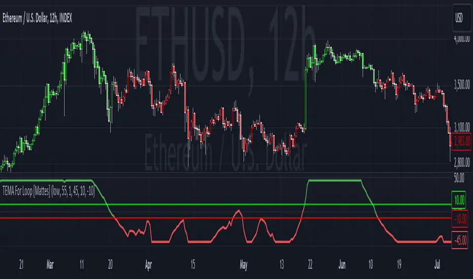
TEMA For Loop [Mattes]The TEMA For Loop indicator is a powerful tool designed for technical analysis, combining the Triple Exponential Moving Average (TEMA) with a custom scoring mechanism based on a for loop. It evaluates price trends over a specified period, allowing traders to identify potential entry and exit points in the market. This indicator enhances decision-making by providing visual cues through dynamic candle coloring, reflecting market sentiment and trends effectively.
Technical Details:
Triple Exponential Moving Average (TEMA):
- TEMA is known for its responsiveness to price changes, as it reduces lag compared to traditional moving averages. The TEMA calculation employs three nested Exponential Moving Averages (EMAs) to produce a smoother trend line, which helps traders identify the direction and momentum of the market.
Scoring Mechanism:
- The scoring mechanism is based on a custom for loop that compares the current TEMA value to previous values over a specified range. The loop counts how many previous values are less than the current value, generating a score that reflects the strength of the trend:
- A higher score indicates a stronger upward trend.
- A lower (negative) score suggests a downward trend.
Threshold Levels:
- Upper Threshold: A score above this level signals a potential long entry, indicating strong bullish momentum.
- Lower Threshold: A score below this level indicates a potential short entry, suggesting bearish sentiment.
>>>These thresholds are adjustable, allowing traders to fine-tune their strategy according to their risk tolerance and market conditions.
Signal Logic:
- The indicator provides clear signals for entering long or short positions based on the score crossing the defined thresholds.
>>Long Entry Signal: When the smoothed score crosses above the upper threshold.
>>Short Entry Signal: When the smoothed score crosses below the lower threshold.
Why This Indicator Is Useful:
>>> Enhanced Decision-Making: The TEMA For Loop indicator offers traders a clear and objective view of market trends, reducing the emotional aspect of trading. By visualizing bullish and bearish conditions, it assists traders in making timely decisions.
>>> Customizable Parameters: The ability to adjust TEMA period, thresholds, and other settings allows traders to tailor the indicator to their specific trading strategies and market conditions.
Visual Clarity: The integration of dynamic candle coloring provides immediate visual cues about the prevailing trend, making it easier for traders to spot potential trade opportunities at a glance.
The TEMA For Loop - Smoothed with Candle Colors indicator is a sophisticated trading tool that utilizes TEMA and a custom scoring mechanism to identify and visualize market trends effectively. By employing dynamic candle coloring, traders gain immediate insights into market sentiment, enabling informed decision-making for entry and exit strategies. This indicator is designed for traders seeking a systematic approach to trend analysis, enhancing their trading performance through clear, actionable signals.
Search in scripts for "Exponential Moving Average"
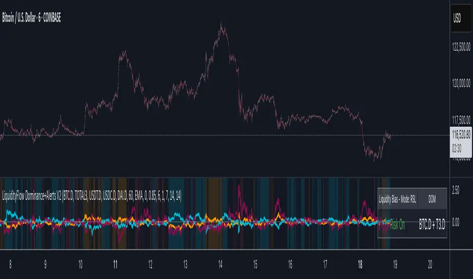
LiquidityFlow Dominance+Alerts (btc.d, T3, Stables)LiquidityFlow Dominance+Alerts: Overview & Usage Guide
Overview
The LiquidityFlow Dominance+Alerts indicator provides a dynamic view of liquidity flow across Bitcoin, Altcoins, and Stablecoins, helping track liquidity shifts and identify market sentiment. By integrating moving averages, custom alerts, and thresholds for extreme outliers, this indicator helps to anticipate bullish and bearish shifts in liquidity and alert market tops and bottoms.
Key features include:
1. Liquidity Flow Monitoring : Track liquidity flow across Bitcoin (BTC), Altcoins (TOTAL3), and Stablecoins (USDT, USDC, DAI).
2. Custom Alerts : Set alerts for key liquidity shifts and extreme conditions in Stablecoin dominance, both with static and moving average (MA)-based calculations.
3. Moving Averages : Use Simple, Exponential, or Weighted Moving Averages to smooth out market data for more reliable signals.
4. Outlier Detection : Identify potential tops and bottoms using thresholds for Stablecoin dominance, with alerts for extreme movements.
Functionality
Data Inputs and Key Metrics
- Symbols Monitored:
- Bitcoin Dominance (BTC.D)
- Altcoin Market Cap (TOTAL3)
- Stablecoins (USDT.D, USDC.D, DAI.D)
- Liquidity Flow Conditions:
- Track percentage changes in dominance across sectors to detect liquidity flow into Bitcoin, Altcoins, or Stablecoins.
- Custom Metrics:
- Liquidity Flow Index: BTC Dominance minus Stablecoin Dominance.
- Liquidity Flow Ratio: BTC Dominance divided by the combined dominance of Stablecoins and Altcoins.
Moving Average Integration
- Select from SMA, EMA, or WMA to apply moving averages to the dominance metrics. Moving averages help smooth out short-term volatility and provide more consistent signals.
- Moving averages are applied to each sector (BTC, Altcoins, and Stablecoins) and compared to their previous period values to determine shifts in liquidity.
Alerts and Thresholds
- % Change Lookback Period: Adjust the lookback period to align with the timeframe of your chart. Shorter timeframes may require a lower lookback period, while higher timeframes may benefit from longer periods.
- Stables Bull/Bear % for Alerts: Set a threshold for when Stablecoin dominance becomes a bullish or bearish signal relative to BTC and Altcoins. A higher threshold may be used in volatile markets to filter out noise.
- Extreme Outliers Detection: Use the **Stables Up/Down Extreme Threshold** to identify potential market tops or bottoms when Stablecoin dominance deviates significantly from historical trends. The **Extreme Lookback Period** controls the time window for detecting these anomalies.
How to Use the Indicator
Adjusting the % Change Lookback Period
- The `% Change Lookback Period` should be adjusted based on your chart’s timeframe. For example, a shorter period (e.g., 7) works well for intraday charts, while longer periods (e.g., 14) might be more suitable for daily or weekly charts.
Setting Thresholds for Alerts
- Stables Bull/Bear % for Alerts: Adjust this setting to define when Stablecoin dominance triggers bullish or bearish alerts. A value like 1% could be a good starting point for most market conditions but can be fine-tuned based on volatility.
- Extreme Lookback Period: Define the lookback period for detecting extreme moves in Stablecoin dominance. This will help identify major tops and bottoms in the market. For shorter-term trades, consider using a shorter extreme lookback (e.g., 7-10 periods).
Alerts for Liquidity Shifts
- The indicator supports alerts for key liquidity shifts, which are useful for staying ahead of market movements. Alerts can be set to notify you when liquidity moves into:
- Bitcoin: Indicating a potential bullish trend for Bitcoin.
- Altcoins: Signaling altcoins are bullish.
- Stablecoins: Suggesting a risk-off environment or market correction.
Extreme Alerts for Stables
- Extreme Up/Down Alerts: These are triggered when Stablecoin dominance crosses extreme thresholds. For example, if Stablecoin dominance rises more than 14% over a set period, it could signal a market top, while a significant drop could indicate a market bottom.
Moving Average Calculations
- In addition to static percentage changes, moving averages can be applied to smooth out dominance values. The type and length of the moving average can be customized:
- SMA (Simple Moving Average): Best for smoothing out volatility in a linear way.
- EMA (Exponential Moving Average): More responsive to recent data, making it useful in faster markets.
- WMA (Weighted Moving Average): Emphasizes more recent data, but less reactive than the EMA.
Additional Usage Tips:
- Background Colors: The indicator visually highlights the dominant liquidity flow:
- Orange: Liquidity is shifting toward Bitcoin.
- Aqua: Liquidity is flowing into Altcoins.
- Red: Liquidity is moving into Stablecoins.
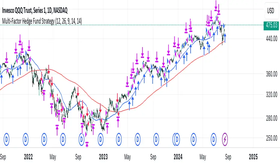
Multi-Factor StrategyThis trading strategy combines multiple technical indicators to create a systematic approach for entering and exiting trades. The goal is to capture trends by aligning several key indicators to confirm the direction and strength of a potential trade. Below is a detailed description of how the strategy works:
Indicators Used
MACD (Moving Average Convergence Divergence):
MACD Line: The difference between the 12-period and 26-period Exponential Moving Averages (EMAs).
Signal Line: A 9-period EMA of the MACD line.
Usage: The strategy looks for crossovers between the MACD line and the Signal line as entry signals. A bullish crossover (MACD line crossing above the Signal line) indicates a potential upward movement, while a bearish crossover (MACD line crossing below the Signal line) signals a potential downward movement.
RSI (Relative Strength Index):
Usage: RSI is used to gauge the momentum of the price movement. The strategy uses specific thresholds: below 70 for long positions to avoid overbought conditions and above 30 for short positions to avoid oversold conditions.
ATR (Average True Range):
Usage: ATR measures market volatility and is used to set dynamic stop-loss and take-profit levels. A stop loss is set at 2 times the ATR, and a take profit at 3 times the ATR, ensuring that risk is managed relative to market conditions.
Simple Moving Averages (SMA):
50-day SMA: A short-term trend indicator.
200-day SMA: A long-term trend indicator.
Usage: The strategy uses the relationship between the 50-day and 200-day SMAs to determine the overall market trend. Long positions are taken when the price is above the 50-day SMA and the 50-day SMA is above the 200-day SMA, indicating an uptrend. Conversely, short positions are taken when the price is below the 50-day SMA and the 50-day SMA is below the 200-day SMA, indicating a downtrend.
Entry Conditions
Long Position:
-MACD Crossover: The MACD line crosses above the Signal line.
-RSI Confirmation: RSI is below 70, ensuring the asset is not overbought.
-SMA Confirmation: The price is above the 50-day SMA, and the 50-day SMA is above the 200-day SMA, indicating a strong uptrend.
Short Position:
MACD Crossunder: The MACD line crosses below the Signal line.
RSI Confirmation: RSI is above 30, ensuring the asset is not oversold.
SMA Confirmation: The price is below the 50-day SMA, and the 50-day SMA is below the 200-day SMA, indicating a strong downtrend.
Opposite conditions for shorts
Exit Strategy
Stop Loss: Set at 2 times the ATR from the entry price. This dynamically adjusts to market volatility, allowing for wider stops in volatile markets and tighter stops in calmer markets.
Take Profit: Set at 3 times the ATR from the entry price. This ensures a favorable risk-reward ratio of 1:1.5, aiming for higher rewards on successful trades.
Visualization
SMAs: The 50-day and 200-day SMAs are plotted on the chart to visualize the trend direction.
MACD Crossovers: Bullish and bearish MACD crossovers are highlighted on the chart to identify potential entry points.
Summary
This strategy is designed to align multiple indicators to increase the probability of successful trades by confirming trends and momentum before entering a position. It systematically manages risk with ATR-based stop loss and take profit levels, ensuring that trades are exited based on market conditions rather than arbitrary points. The combination of trend indicators (SMAs) with momentum and volatility indicators (MACD, RSI, ATR) creates a robust approach to trading in various market environments.
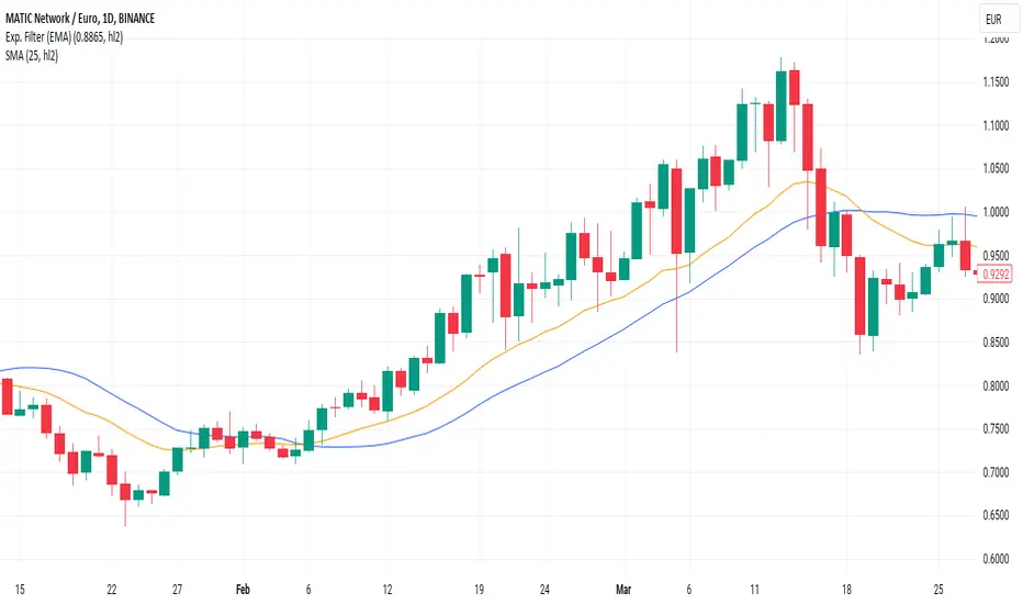
Exponential Smoothing FilterThe digital exponential filter, in finance known as Exponential Moving Average (EMA) , can be used as a technical indicator for chart analysis to visualize uptrends and downtrends in the market. Unlike the classic simple moving average, the EMA requires only two values for its calculation: the last calculated exponential average price and the current price. This is a simple and fast calculation - even for wide smoothing windows. For further details and the math please refer to the "exponential smoothing" article on Wikipedia.
Here are some additional key points about the exponential moving average:
The EMA can react more quickly to price changes because it can give more weight to current prices - depending on your parameter settings.
Short-term, disruptive price fluctuations are smoothed out well, making prevailing trends more visible.
Despite good smoothing properties, it delays the input values slightly, so it can follow sudden trend changes well.
The EMA is well suited to dynamic markets and trading strategies.
The filter is a good basis for further processing such as gradient analysis.
How to use
When you add the script to your charts, you'll immediately see a thin orange line across your time series, smoothing out price fluctuations.
There are only two parameters to set
smoothing factor between 0.0000 = no smoothing and 0.9999 = strong smoothing
input source : open, high, low, close hl2, etc.
Chart output
In the example chart above, you can see that the orange line follows the highs and lows better than the blue line , which is a simple moving average (SMA).
Additionally, the orange line has a shorter lag, or reacts faster when the trend of the original price data suddenly changes. These characteristics are critical for buying and selling decisions: quickly reacting and tracking highs and lows while providing a smooth line that filters out distracting noise.
SRTL, 2EMA & TRAMASRTL - Support Resistance and Trend Line with Double EMA and TRAMA
The SRTL indicator is a powerful tool for technical analysis that seamlessly integrates support and resistance levels, trend lines, and moving average signals. It offers traders a comprehensive view of the market's dynamics, making it a valuable addition to any trading toolkit. Here's a concise summary of its key features and functionalities:
Key Features:
- Dynamic Support and Resistance Levels based on Pivot Points
- Trend Lines based on Recent Pivot Points
- Double Exponential Moving Averages (EMA) with adjustable lengths
- Trend Regularity Adaptive Moving Average (TRAMA) for trend identification
- Buy and Sell signals based on the crossover of EMAs
The indicator is composed of 4 main components:
1. Support and resistance levels: The indicator calculates support and resistance levels based on pivot points and a channel width parameter. These levels can be used to identify potential entry and exit points for trades. The script calculates and plots dynamic support and resistance levels based on pivot points. Users can adjust the period for calculating pivot points, loopback period, and S/R strength to customize the levels' sensitivity.
2. Trend Lines: The script identifies and plots trend lines based on recent pivot points. Users can customize the number of pivot points to consider and the start date to begin plotting the trend lines. The script identifies and plots trend lines based on recent pivot points. By adjusting the number of pivot points to consider and the start date, traders can visualize potential trends and assess the market's overall direction. This feature helps traders understand the prevailing market sentiment and make informed trading decisions.
3. Double Exponential Moving Averages (EMA): The script calculates and plots two Exponential Moving Averages (EMA) with customizable lengths. A crossover of these EMAs can be used as a signal for potential trend changes. The study calculates and displays two Exponential Moving Averages (EMA) with adjustable lengths. The crossover of these EMAs serves as a crucial signal for potential trend changes. When the faster EMA crosses above the slower EMA, a "Buy" signal is generated, and when the faster EMA crosses below the slower EMA, a "Sell" signal is generated.
4. Trend Regularity Adaptive Moving Average (TRAMA): The script calculates and plots the TRAMA, a unique adaptive moving average that helps identify trends and adapt to market conditions. The indicator includes the Trend Regularity Adaptive Moving Average (TRAMA), an adaptive moving average designed to identify trends and adapt to varying market conditions. TRAMA helps traders gauge the strength of a trend and provides valuable insights into potential trend reversals.
5. Signals: The script generates "Buy - Green" and "Sell- Red" signals based on the crossover of the two EMAs and Pivot Point Trend Levels. That Also Customizable.
How to Use:
The SRTL indicator is a powerful tool for technical analysis, offering multiple layers of information for traders. When the price approaches dynamic support or resistance levels, The dynamic support and resistance levels are based on pivot points and adjust to the market's current conditions. The trend lines help visualize potential trends and can be adjusted to show different numbers of pivot points. Additionally, the Double EMA and TRAMA lines provide further insight into the market's momentum and potential reversals. Traders can assess the potential for trend reversals or breakouts. The trend lines help visualize the market's prevailing direction, and the crossover of the Double EMA signals potential entry and exit points.
Traders should use this study as part of a broader trading strategy and combine it with other technical indicators, fundamental analysis, and risk management techniques. Additionally, it's essential to test the indicator thoroughly in a demo or back testing environment before applying it to live trading to ensure its compatibility with individual trading styles and preferences.

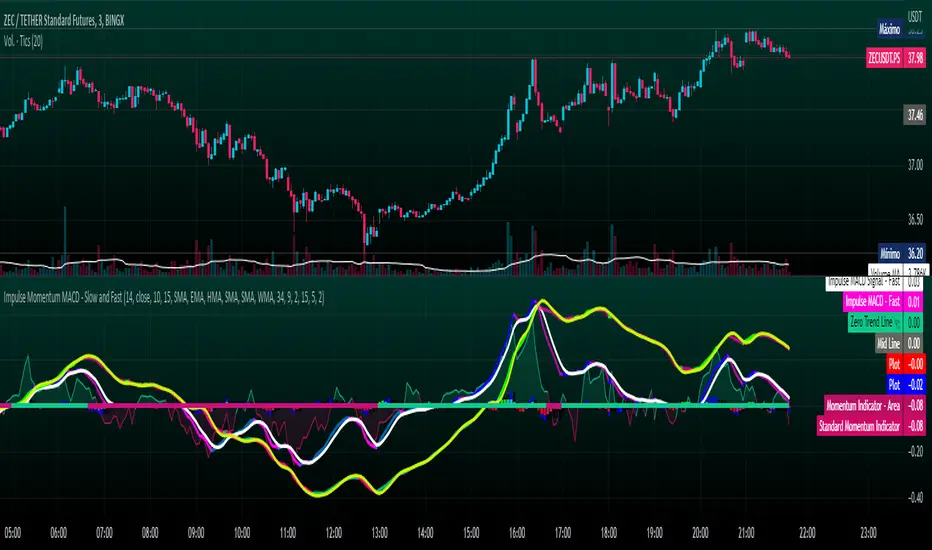
Impulse Momentum MACD - Slow and FastImpulse Momentum MACD - Slow and Fast
The Momentum indicator is a technical indicator that measures the speed and strength of the price movement of a financial asset. This indicator is used to identify the underlying strength of a trend and predict potential changes in price direction, when the indicator crosses the zero line, it can signal a change of direction in the price trend.
On the other hand, the MACD is an indicator used to identify the trend and strength of the market and shows the difference between two exponential moving averages ( EMA ) of different periods. The MACD is commonly used to determine the direction of an asset's price trend.
COPOSITION AND USE OF THE INDICATOR
This script is an implementation of the Impulse Momentum MACD indicator with two variations: slow and fast. It uses a combination of the Momentum indicator and the Moving Average Convergence/Divergence (MACD) indicator to identify trend reversals and momentum changes in an asset's price.
The combination of both indicators can help traders identify market entry and exit opportunities. The Impulse Momentum MACD is a Modified MACD, it is formed by filtering the values in a range of Modifiable Moving Averages by calculating their high and low ranges,This indicator has two parts: a slow part and a fast part. The slow part uses input values for the lengths of the moving averages and the length of the signal for the MACD indicator. The fast part uses different input values for the lengths of the moving averages. Also, each part has its own set of line colors and histogram colors for easy visualization.
The script also includes inputs to choose the type of moving average to use (SMA, EMA, etc.), the lookback period, the colors for the histogram lines and bars, and a zero trend line (also known as a horizontal trend line). ).
* Highest performing custom settings for the zero trend line. For Operations of:
- One Minute: Trend Line Time Frame = Five Minutes.
- Three Minutes: Trend Line Time Frame = Fifteen Minutes.
- Five Minutes: Trend Line Time Frame = Thirty Minutes.
- Fifteen Minutes: Trend Line Time Frame = Sixty Minutes.
Rules For Trading
🔹 Bullish:
* The Zero Horizontal Trend Line should be in Green Color.
* The Slow Histogram Bar should be in Green Color.
* The Fast Histogram Bar must be in Blue or Black Color or No Bar Appears.
* The Momentum Line or Momentum Area must be in Green Color.
crosses:
- When the Impulse Momentum MACD Slow line crosses the Impulse Momentum MACD Slow signal line upwards.
- When the Impulse Momentum MACD Fast line crosses the Impulse Momentum MACD Fast signal line upwards.
- Note 1: A Position is Opened when the condition of any of the aforementioned crossovers is met.
- Note 2: If the two aforementioned crossings anticipate the condition of the Zero Horizontal Tendency Line because it is in Red; A position is only opened immediately when the Zero Horizontal Trend line turns Green.
🔹 Bearish:
* The Zero Horizontal Trend Line should be in Red Color.
* The Slow Histogram Bar should be in Red Color.
* The Fast Histogram Bar must be in Blue or Black Color or No Bar Appears.
* The Momentum Line or Momentum Area must be in Red Color.
crosses:
- When the Impulse Momentum MACD Slow line crosses the Impulse Momentum MACD Slow signal line downwards.
- When the Impulse Momentum MACD Fast line crosses the Impulse Momentum MACD Fast signal line downwards.
- Note 1: A Position is Opened when the condition of any of the aforementioned crossovers is met.
- Note 2: If the two aforementioned crossings anticipate the condition of the Zero Horizontal Tendency Line because it is Green, an immediate position is only opened when the Zero Horizontal Tendency line turns Red.
This script can be used in different markets such as forex, indices and cryptocurrencies for analysis and trading. However, it is important to note that no trading strategy is guaranteed to be profitable, and traders should always conduct their own research and risk management.
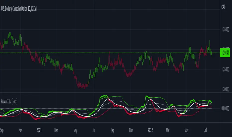
PA-Adaptive MACD w/ Variety Levels [Loxx]PA-Adaptive MACD w/ Variety Levels is a Phase Accumulation Adaptive MACD with both floating and quantile levels. This is tuned for Forex. You'll have to adjust the Phase Accumulation Cycle settings to work for crypto and stock markets.
What is MACD?
Moving average convergence divergence ( MACD ) is a trend-following momentum indicator that shows the relationship between two moving averages of a security’s price. The MACD is calculated by subtracting the 26-period exponential moving average ( EMA ) from the 12-period EMA .
What is the Phase Accumulation Cycle?
The phase accumulation method of computing the dominant cycle is perhaps the easiest to comprehend. In this technique, we measure the phase at each sample by taking the arctangent of the ratio of the quadrature component to the in-phase component. A delta phase is generated by taking the difference of the phase between successive samples. At each sample we can then look backwards, adding up the delta phases.When the sum of the delta phases reaches 360 degrees, we must have passed through one full cycle, on average.The process is repeated for each new sample.
The phase accumulation method of cycle measurement always uses one full cycle’s worth of historical data.This is both an advantage and a disadvantage.The advantage is the lag in obtaining the answer scales directly with the cycle period.That is, the measurement of a short cycle period has less lag than the measurement of a longer cycle period. However, the number of samples used in making the measurement means the averaging period is variable with cycle period. longer averaging reduces the noise level compared to the signal.Therefore, shorter cycle periods necessarily have a higher out- put signal-to-noise ratio.
Included:
Zero-line and signal cross options for bar coloring, signals, and alerts
Alerts
Signals
Loxx's Expanded Source Types
4 moving average types
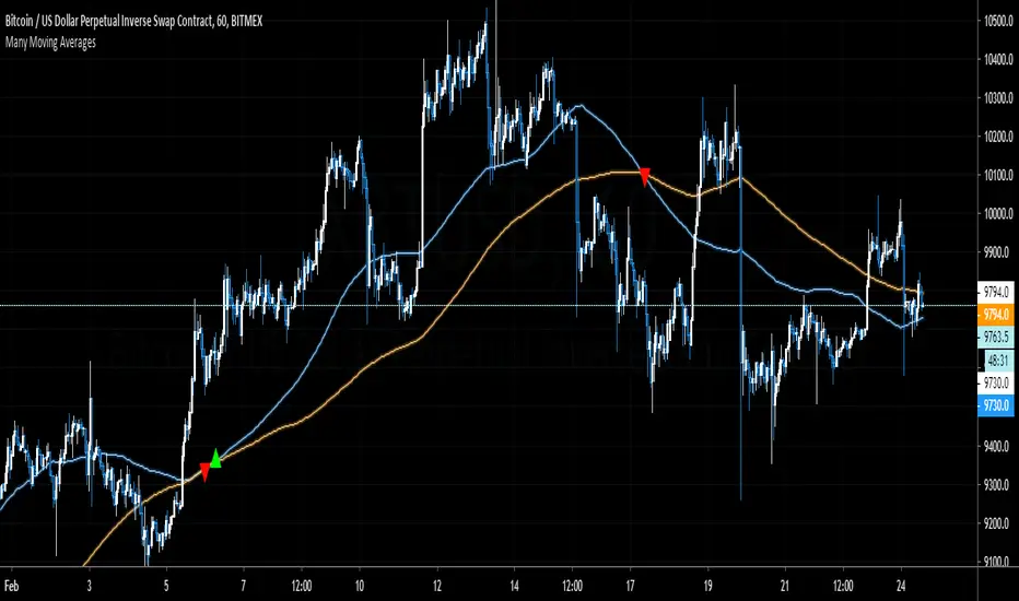
Many Moving AveragesThis script allows you to add two moving averages to a chart, where the type of moving average can be chosen from a collection of 15 different moving average algorithms. Each moving average can also have different lengths and crossovers/unders can be displayed and alerted on.
The supported moving average types are:
Simple Moving Average ( SMA )
Exponential Moving Average ( EMA )
Double Exponential Moving Average ( DEMA )
Triple Exponential Moving Average ( TEMA )
Weighted Moving Average ( WMA )
Volume Weighted Moving Average ( VWMA )
Smoothed Moving Average ( SMMA )
Hull Moving Average ( HMA )
Least Square Moving Average/Linear Regression ( LSMA )
Arnaud Legoux Moving Average ( ALMA )
Jurik Moving Average ( JMA )
Volatility Adjusted Moving Average ( VAMA )
Fractal Adaptive Moving Average ( FRAMA )
Zero-Lag Exponential Moving Average ( ZLEMA )
Kauman Adaptive Moving Average ( KAMA )
Many of the moving average algorithms were taken from other peoples' scripts. I'd like to thank the authors for making their code available.
JayRogers
Alex Orekhov (everget)
Alex Orekhov (everget)
Joris Duyck (JD)
nemozny
Shizaru
KobySK
Jurik Research and Consulting for inventing the JMA.
Educational Trend Direction (Up & Down)🔍 Overview
This indicator is designed to visually represent trend direction and trend transitions using a simple moving-average relationship. It is built strictly for educational and analytical purposes, allowing users to observe how price behaves during upward and downward market phases without relying on trading signals or predictions.
The indicator focuses on trend context, not trade execution.
⚙️ How the Indicator Works
The script calculates two exponential moving averages:
A fast trend line that reacts quickly to recent price changes
A slow trend line that represents broader market direction
Trend direction is determined by the relative position of these two lines.
When the fast line moves above the slow line, the market is considered to be in an upward trend phase
When the fast line moves below the slow line, the market is considered to be in a downward trend phase
This relationship helps visualize trend shifts and momentum changes in a simple and intuitive way.
🎨 Visual Components Explained
🟢 Green Trend Line
Represents the fast moving average during upward trend phases
Indicates that price is maintaining strength relative to the broader trend
Color reflects trend direction only, not confirmation or entry
🔴 Red Trend Line
Represents the fast moving average during downward trend phases
Indicates sustained weakness relative to the broader trend
Color does not imply selling or future continuation
⚪ Grey Trend Line
Represents the slow moving average
Acts as a baseline trend reference
Helps distinguish between short-term fluctuations and broader direction
🎨 Background Shading
Light green shading appears during upward trend environments
Light red shading appears during downward trend environments
Background color provides context only and does not signal market actions
🎯 Purpose & Benefits
Helps identify trend phases in a clear and minimal way
Improves understanding of trend transitions and momentum shifts
Reduces visual noise compared to raw price data
Encourages context-based analysis instead of signal dependency
Suitable for all markets and timeframes
⚠️ Important Notes
This indicator does not generate buy or sell signals
No targets, stop levels, or performance metrics are included
Trend conditions are descriptive, not predictive
Past behavior does not guarantee future outcomes
Users should always apply their own analysis and risk management when interpreting market data.
📚 Intended Use
This tool is intended for:
Market trend study
Educational demonstrations
Visual analysis of trend direction
Long-term chart structure awareness
It is not intended for automated trading or decision-making.

Neeson Vegas ChannelVegas Channel Indicator: A Comprehensive Multi-Timeframe Trend-Following System
Originality and Conceptual Foundation
This script implements an enhanced version of the classic "Vegas Tunnel" or "Vegas Channel" methodology, popularized by traders who follow the work associated with the "Vegas" technique. Its primary original contribution lies in its specific, rule-based multi-layered trend identification and visualization system. While the core uses well-known Exponential Moving Averages (EMAs), the originality is in the precise combination of periods and the strict, hierarchical logic for defining trend states and generating signals.
Unlike simpler moving average crossovers or single-tunnel systems, this script employs three distinct EMA pairs, each serving a unique purpose within the trend hierarchy:
Short-Term Momentum Pair (EMA 12 & 24): Acts as the primary signal trigger and momentum gauge.
Core Trend Tunnel (EMA 144 & 169): Serves as the central "channel" or "tunnel." A key visual and logical component is the shading between these two lines, which thickens and changes color with the trend, creating a dynamic channel.
Long-Term Foundation Pair (EMA 580 & 670): Represents the underlying, slower-moving trend foundation, providing context for the higher-timeframe bias.
The system's true innovation is its binary and exclusive trend definition logic. It does not rely on a single crossover. Instead, it defines a confirmed Uptrend only when both the short-term EMAs (12 and 24) are established above both lines of the core tunnel (144 and 169). Conversely, a Downtrend is confirmed only when both short-term EMAs are established below both core tunnel lines. This creates a high-confidence filter, reducing whipsaw signals that can occur when price oscillates around a single moving average.
Functionality, Implementation, and Usage
What It Does:
This indicator is a multi-timeframe trend identification and signal-generation tool. It visually condenses trend information from short, medium, and long-term perspectives onto a single chart. Its primary functions are:
Trend State Classification: It dynamically classifies the market into one of three states: Bull Trend (Blue), Bear Trend (Orange), or Sideways/Congestion (Gray). This is reflected in the chart's background color, the color of all EMA lines, and the fill of the central 144/169 channel.
Signal Generation: It plots discrete buy and sell arrows. A Buy Signal (blue upward triangle) appears the first bar the market transitions into the defined "Uptrend" state from a non-uptrend state. A Sell Signal (orange downward triangle) appears the first bar the market transitions into the defined "Downtrend" state.
Visual Structuring: It plots all six EMAs and prominently highlights the interaction zone between the 144 and 169 EMAs with a colored fill, making the "tunnel" a focal point for support/resistance and trend quality assessment.
How It's Implemented:
The logic is implemented through a clear sequence of conditional checks:
Calculation: All six EMAs are calculated based on user-definable periods (defaults as listed).
Trend Logic: The script continuously evaluates the position of EMA12 and EMA24 relative to EMA144 and EMA169 using strict AND conditions to define the uptrend and downtrend Boolean variables.
Signal Logic: A signal (buy or sell) is generated only on the change of the trend state. It uses a check of the form current_trend_state AND (NOT previous_bar_trend_state) to pinpoint the exact bar of transition.
Visual Feedback: All plot colors, the channel fill color, and the background color are unified and determined by the current trend state variable. Labels for the trend and each EMA line are drawn on the last bar for clarity.
How to Use It:
Traders employ this indicator primarily for trend-following and breakout confirmation. It is suited for swing trading or higher-timeframe positional trades rather than scalping, due to the lag inherent in its longer EMAs and its focus on confirmed states.
Trend Bias: The overall color scheme (blue/orange/gray background) provides an immediate, at-a-glance assessment of the dominant trend force. Trading in the direction of the colored background is considered aligned with the system's trend.
Signal Entry: The arrow signals are not meant for blind entry. They mark the point of a confirmed trend state transition.
A Buy Signal suggests the short-term momentum (12,24) has decisively broken above and established itself over the medium-term trend framework (144,169). This could be used as a trigger for long entries, preferably with the long-term EMAs (580,670) sloping upwards or flat, adding confluence.
A Sell Signal suggests the opposite breakdown.
Channel as Dynamic S/R: The filled area between EMA144 and EMA169 acts as a dynamic support zone in an uptrend and a resistance zone in a downtrend. Pullbacks into this "tunnel" that hold without triggering a sell signal (i.e., without both EMA12 & 24 closing back below both tunnel lines) can be viewed as potential continuation opportunities.
Filter for Other Systems: The clear trend state (uptrend/downtrend) can be exported or used as a filter for other trading systems or discretionary decisions, ensuring actions are only taken in the direction of the script's defined trend.
Core Computational Philosophy and Strategic Rationale
The script's logic is rooted in the philosophy of trend hierarchy and confirmation. It belongs to the category of Multi-Moving Average Convergence/Divergence Systems with State-Based Rules.
The 144/169 Tunnel: These numbers are derived from Fibonacci sequences (144, 169 is 12^2 and 13^2). They are believed by proponents to represent a natural rhythm or "heartbeat" of the market, defining a robust intermediate-term trend framework.
The 12/24 Pair: A standard fast-moving average pair commonly used to gauge short-term momentum and trigger entries.
The Strategic Innovation (Dual-Condition Crossover): The core idea is that a crossover of a single fast MA above a single slow MA can be false and noisy. By requiring both members of a fast pair to establish position relative to both members of a slower "tunnel" pair, the system demands a broader, more concerted move. This seeks to filter out weak, unsustainable breaks and only capture shifts in momentum strong enough to flip the entire short-term structure's position relative to the medium-term structure.
The 580/670 Pair: These very slow EMAs represent the "secular" trend. While not part of the direct signal logic, they provide critical context. A buy signal that occurs while price is above the 580/670 pair (which would be sloping up in a healthy bull market) carries more weight than one that occurs while price is below this long-term foundation, which might indicate a counter-trend rally.
In essence, this script is more than just moving averages on a chart. It is a systematic, rule-based framework for identifying when the market's short-term energy (12,24) has converged sufficiently to overcome and reposition itself against its medium-term equilibrium (144/169 tunnel), thereby signaling a high-probability phase change in trend, all while considering the backdrop of a long-term trend (580/670).

FatihStrategy: Universal Pivot System v3.3.1FatihStrategy: Universal Pivot System v3.3.1 is an advanced technical analysis indicator that combines multi-timeframe pivot averages with EMA trend filters in a single visual system.
🔹 How It Works
Depending on the selected pivot mode, the indicator calculates and visualizes:
Daily & 3-Day Average Pivots
Weekly & 3-Week Average Pivots
Monthly & 3-Month Average Pivots
Yearly & 3-Year Average Pivots
The difference between pivot levels is displayed as colored boxes:
Red Box → Lower timeframe pivot zone
Yellow Box → Higher timeframe pivot zone
These zones help identify potential support, resistance, and consolidation areas.
🔹 EMA Trend Support
Optional exponential moving averages:
20 EMA
50 EMA
200 EMA
can be enabled to assist with trend direction and trade filtering.
🔹 Suitable For
Day traders and swing traders
Pivot-based strategies
Traders looking for clear visual support/resistance zones
Crypto, forex, and stock market analysis
⚠️ Disclaimer
This indicator is not financial advice.
Always use proper risk management and confirm signals with your own trading strategy.

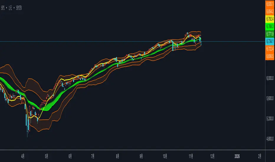
双布林Dual Bollinger Bands
This technical indicator combines dual Bollinger Bands with multiple moving average overlays to provide a comprehensive view of price trends, volatility, and potential support/resistance zones.
**Components:**
1. **TEMA21 (Triple Exponential Moving Average)**
- Yellow line representing the 21-period TEMA
- Provides smooth trend direction with reduced lag compared to traditional moving averages
- Calculated using three sequential EMAs to filter out market noise
2. **SMA21 & EMA21 Channel**
- Green filled area between the 21-period Simple Moving Average and Exponential Moving Average
- Visualizes the dynamic zone where these two averages interact
- Helps identify trend strength when price stays above/below this channel
3. **MA21 (Simple Moving Average)**
- Bright green line showing the 21-period SMA
- Classic trend-following indicator
4. **EMA21 (Exponential Moving Average)**
- Dark green line displaying the 21-period EMA
- More responsive to recent price changes than SMA
5. **Dual Bollinger Bands**
- **Outer Bands (2 Standard Deviations)**: Orange lines marking the traditional Bollinger Band boundaries
- **Inner Bands (1 Standard Deviation)**: Orange lines creating a tighter volatility zone
- **Orange Shaded Areas**: Highlight the zones between outer and inner bands
- All bands use a 21-period basis and are fully customizable
**Settings:**
- Length: 21 (adjustable)
- Source: Close price (adjustable)
- Outer Band StdDev: 2.0 (adjustable)
- Inner Band StdDev: 1.0 (adjustable)
- Offset: 0 (adjustable from -500 to +500)
**Usage:**
This indicator is ideal for identifying trend direction, volatility expansion/contraction, and potential reversal zones. The dual Bollinger Bands provide multiple levels for support/resistance analysis, while the moving averages confirm trend strength and direction.
Markov Chain [3D] | FractalystWhat exactly is a Markov Chain?
This indicator uses a Markov Chain model to analyze, quantify, and visualize the transitions between market regimes (Bull, Bear, Neutral) on your chart. It dynamically detects these regimes in real-time, calculates transition probabilities, and displays them as animated 3D spheres and arrows, giving traders intuitive insight into current and future market conditions.
How does a Markov Chain work, and how should I read this spheres-and-arrows diagram?
Think of three weather modes: Sunny, Rainy, Cloudy.
Each sphere is one mode. The loop on a sphere means “stay the same next step” (e.g., Sunny again tomorrow).
The arrows leaving a sphere show where things usually go next if they change (e.g., Sunny moving to Cloudy).
Some paths matter more than others. A more prominent loop means the current mode tends to persist. A more prominent outgoing arrow means a change to that destination is the usual next step.
Direction isn’t symmetric: moving Sunny→Cloudy can behave differently than Cloudy→Sunny.
Now relabel the spheres to markets: Bull, Bear, Neutral.
Spheres: market regimes (uptrend, downtrend, range).
Self‑loop: tendency for the current regime to continue on the next bar.
Arrows: the most common next regime if a switch happens.
How to read: Start at the sphere that matches current bar state. If the loop stands out, expect continuation. If one outgoing path stands out, that switch is the typical next step. Opposite directions can differ (Bear→Neutral doesn’t have to match Neutral→Bear).
What states and transitions are shown?
The three market states visualized are:
Bullish (Bull): Upward or strong-market regime.
Bearish (Bear): Downward or weak-market regime.
Neutral: Sideways or range-bound regime.
Bidirectional animated arrows and probability labels show how likely the market is to move from one regime to another (e.g., Bull → Bear or Neutral → Bull).
How does the regime detection system work?
You can use either built-in price returns (based on adaptive Z-score normalization) or supply three custom indicators (such as volume, oscillators, etc.).
Values are statistically normalized (Z-scored) over a configurable lookback period.
The normalized outputs are classified into Bull, Bear, or Neutral zones.
If using three indicators, their regime signals are averaged and smoothed for robustness.
How are transition probabilities calculated?
On every confirmed bar, the algorithm tracks the sequence of detected market states, then builds a rolling window of transitions.
The code maintains a transition count matrix for all regime pairs (e.g., Bull → Bear).
Transition probabilities are extracted for each possible state change using Laplace smoothing for numerical stability, and frequently updated in real-time.
What is unique about the visualization?
3D animated spheres represent each regime and change visually when active.
Animated, bidirectional arrows reveal transition probabilities and allow you to see both dominant and less likely regime flows.
Particles (moving dots) animate along the arrows, enhancing the perception of regime flow direction and speed.
All elements dynamically update with each new price bar, providing a live market map in an intuitive, engaging format.
Can I use custom indicators for regime classification?
Yes! Enable the "Custom Indicators" switch and select any three chart series as inputs. These will be normalized and combined (each with equal weight), broadening the regime classification beyond just price-based movement.
What does the “Lookback Period” control?
Lookback Period (default: 100) sets how much historical data builds the probability matrix. Shorter periods adapt faster to regime changes but may be noisier. Longer periods are more stable but slower to adapt.
How is this different from a Hidden Markov Model (HMM)?
It sets the window for both regime detection and probability calculations. Lower values make the system more reactive, but potentially noisier. Higher values smooth estimates and make the system more robust.
How is this Markov Chain different from a Hidden Markov Model (HMM)?
Markov Chain (as here): All market regimes (Bull, Bear, Neutral) are directly observable on the chart. The transition matrix is built from actual detected regimes, keeping the model simple and interpretable.
Hidden Markov Model: The actual regimes are unobservable ("hidden") and must be inferred from market output or indicator "emissions" using statistical learning algorithms. HMMs are more complex, can capture more subtle structure, but are harder to visualize and require additional machine learning steps for training.
A standard Markov Chain models transitions between observable states using a simple transition matrix, while a Hidden Markov Model assumes the true states are hidden (latent) and must be inferred from observable “emissions” like price or volume data. In practical terms, a Markov Chain is transparent and easier to implement and interpret; an HMM is more expressive but requires statistical inference to estimate hidden states from data.
Markov Chain: states are observable; you directly count or estimate transition probabilities between visible states. This makes it simpler, faster, and easier to validate and tune.
HMM: states are hidden; you only observe emissions generated by those latent states. Learning involves machine learning/statistical algorithms (commonly Baum–Welch/EM for training and Viterbi for decoding) to infer both the transition dynamics and the most likely hidden state sequence from data.
How does the indicator avoid “repainting” or look-ahead bias?
All regime changes and matrix updates happen only on confirmed (closed) bars, so no future data is leaked, ensuring reliable real-time operation.
Are there practical tuning tips?
Tune the Lookback Period for your asset/timeframe: shorter for fast markets, longer for stability.
Use custom indicators if your asset has unique regime drivers.
Watch for rapid changes in transition probabilities as early warning of a possible regime shift.
Who is this indicator for?
Quants and quantitative researchers exploring probabilistic market modeling, especially those interested in regime-switching dynamics and Markov models.
Programmers and system developers who need a probabilistic regime filter for systematic and algorithmic backtesting:
The Markov Chain indicator is ideally suited for programmatic integration via its bias output (1 = Bull, 0 = Neutral, -1 = Bear).
Although the visualization is engaging, the core output is designed for automated, rules-based workflows—not for discretionary/manual trading decisions.
Developers can connect the indicator’s output directly to their Pine Script logic (using input.source()), allowing rapid and robust backtesting of regime-based strategies.
It acts as a plug-and-play regime filter: simply plug the bias output into your entry/exit logic, and you have a scientifically robust, probabilistically-derived signal for filtering, timing, position sizing, or risk regimes.
The MC's output is intentionally "trinary" (1/0/-1), focusing on clear regime states for unambiguous decision-making in code. If you require nuanced, multi-probability or soft-label state vectors, consider expanding the indicator or stacking it with a probability-weighted logic layer in your scripting.
Because it avoids subjectivity, this approach is optimal for systematic quants, algo developers building backtested, repeatable strategies based on probabilistic regime analysis.
What's the mathematical foundation behind this?
The mathematical foundation behind this Markov Chain indicator—and probabilistic regime detection in finance—draws from two principal models: the (standard) Markov Chain and the Hidden Markov Model (HMM).
How to use this indicator programmatically?
The Markov Chain indicator automatically exports a bias value (+1 for Bullish, -1 for Bearish, 0 for Neutral) as a plot visible in the Data Window. This allows you to integrate its regime signal into your own scripts and strategies for backtesting, automation, or live trading.
Step-by-Step Integration with Pine Script (input.source)
Add the Markov Chain indicator to your chart.
This must be done first, since your custom script will "pull" the bias signal from the indicator's plot.
In your strategy, create an input using input.source()
Example:
//@version=5
strategy("MC Bias Strategy Example")
mcBias = input.source(close, "MC Bias Source")
After saving, go to your script’s settings. For the “MC Bias Source” input, select the plot/output of the Markov Chain indicator (typically its bias plot).
Use the bias in your trading logic
Example (long only on Bull, flat otherwise):
if mcBias == 1
strategy.entry("Long", strategy.long)
else
strategy.close("Long")
For more advanced workflows, combine mcBias with additional filters or trailing stops.
How does this work behind-the-scenes?
TradingView’s input.source() lets you use any plot from another indicator as a real-time, “live” data feed in your own script (source).
The selected bias signal is available to your Pine code as a variable, enabling logical decisions based on regime (trend-following, mean-reversion, etc.).
This enables powerful strategy modularity : decouple regime detection from entry/exit logic, allowing fast experimentation without rewriting core signal code.
Integrating 45+ Indicators with Your Markov Chain — How & Why
The Enhanced Custom Indicators Export script exports a massive suite of over 45 technical indicators—ranging from classic momentum (RSI, MACD, Stochastic, etc.) to trend, volume, volatility, and oscillator tools—all pre-calculated, centered/scaled, and available as plots.
// Enhanced Custom Indicators Export - 45 Technical Indicators
// Comprehensive technical analysis suite for advanced market regime detection
//@version=6
indicator('Enhanced Custom Indicators Export | Fractalyst', shorttitle='Enhanced CI Export', overlay=false, scale=scale.right, max_labels_count=500, max_lines_count=500)
// |----- Input Parameters -----| //
momentum_group = "Momentum Indicators"
trend_group = "Trend Indicators"
volume_group = "Volume Indicators"
volatility_group = "Volatility Indicators"
oscillator_group = "Oscillator Indicators"
display_group = "Display Settings"
// Common lengths
length_14 = input.int(14, "Standard Length (14)", minval=1, maxval=100, group=momentum_group)
length_20 = input.int(20, "Medium Length (20)", minval=1, maxval=200, group=trend_group)
length_50 = input.int(50, "Long Length (50)", minval=1, maxval=200, group=trend_group)
// Display options
show_table = input.bool(true, "Show Values Table", group=display_group)
table_size = input.string("Small", "Table Size", options= , group=display_group)
// |----- MOMENTUM INDICATORS (15 indicators) -----| //
// 1. RSI (Relative Strength Index)
rsi_14 = ta.rsi(close, length_14)
rsi_centered = rsi_14 - 50
// 2. Stochastic Oscillator
stoch_k = ta.stoch(close, high, low, length_14)
stoch_d = ta.sma(stoch_k, 3)
stoch_centered = stoch_k - 50
// 3. Williams %R
williams_r = ta.stoch(close, high, low, length_14) - 100
// 4. MACD (Moving Average Convergence Divergence)
= ta.macd(close, 12, 26, 9)
// 5. Momentum (Rate of Change)
momentum = ta.mom(close, length_14)
momentum_pct = (momentum / close ) * 100
// 6. Rate of Change (ROC)
roc = ta.roc(close, length_14)
// 7. Commodity Channel Index (CCI)
cci = ta.cci(close, length_20)
// 8. Money Flow Index (MFI)
mfi = ta.mfi(close, length_14)
mfi_centered = mfi - 50
// 9. Awesome Oscillator (AO)
ao = ta.sma(hl2, 5) - ta.sma(hl2, 34)
// 10. Accelerator Oscillator (AC)
ac = ao - ta.sma(ao, 5)
// 11. Chande Momentum Oscillator (CMO)
cmo = ta.cmo(close, length_14)
// 12. Detrended Price Oscillator (DPO)
dpo = close - ta.sma(close, length_20)
// 13. Price Oscillator (PPO)
ppo = ta.sma(close, 12) - ta.sma(close, 26)
ppo_pct = (ppo / ta.sma(close, 26)) * 100
// 14. TRIX
trix_ema1 = ta.ema(close, length_14)
trix_ema2 = ta.ema(trix_ema1, length_14)
trix_ema3 = ta.ema(trix_ema2, length_14)
trix = ta.roc(trix_ema3, 1) * 10000
// 15. Klinger Oscillator
klinger = ta.ema(volume * (high + low + close) / 3, 34) - ta.ema(volume * (high + low + close) / 3, 55)
// 16. Fisher Transform
fisher_hl2 = 0.5 * (hl2 - ta.lowest(hl2, 10)) / (ta.highest(hl2, 10) - ta.lowest(hl2, 10)) - 0.25
fisher = 0.5 * math.log((1 + fisher_hl2) / (1 - fisher_hl2))
// 17. Stochastic RSI
stoch_rsi = ta.stoch(rsi_14, rsi_14, rsi_14, length_14)
stoch_rsi_centered = stoch_rsi - 50
// 18. Relative Vigor Index (RVI)
rvi_num = ta.swma(close - open)
rvi_den = ta.swma(high - low)
rvi = rvi_den != 0 ? rvi_num / rvi_den : 0
// 19. Balance of Power (BOP)
bop = (close - open) / (high - low)
// |----- TREND INDICATORS (10 indicators) -----| //
// 20. Simple Moving Average Momentum
sma_20 = ta.sma(close, length_20)
sma_momentum = ((close - sma_20) / sma_20) * 100
// 21. Exponential Moving Average Momentum
ema_20 = ta.ema(close, length_20)
ema_momentum = ((close - ema_20) / ema_20) * 100
// 22. Parabolic SAR
sar = ta.sar(0.02, 0.02, 0.2)
sar_trend = close > sar ? 1 : -1
// 23. Linear Regression Slope
lr_slope = ta.linreg(close, length_20, 0) - ta.linreg(close, length_20, 1)
// 24. Moving Average Convergence (MAC)
mac = ta.sma(close, 10) - ta.sma(close, 30)
// 25. Trend Intensity Index (TII)
tii_sum = 0.0
for i = 1 to length_20
tii_sum += close > close ? 1 : 0
tii = (tii_sum / length_20) * 100
// 26. Ichimoku Cloud Components
ichimoku_tenkan = (ta.highest(high, 9) + ta.lowest(low, 9)) / 2
ichimoku_kijun = (ta.highest(high, 26) + ta.lowest(low, 26)) / 2
ichimoku_signal = ichimoku_tenkan > ichimoku_kijun ? 1 : -1
// 27. MESA Adaptive Moving Average (MAMA)
mama_alpha = 2.0 / (length_20 + 1)
mama = ta.ema(close, length_20)
mama_momentum = ((close - mama) / mama) * 100
// 28. Zero Lag Exponential Moving Average (ZLEMA)
zlema_lag = math.round((length_20 - 1) / 2)
zlema_data = close + (close - close )
zlema = ta.ema(zlema_data, length_20)
zlema_momentum = ((close - zlema) / zlema) * 100
// |----- VOLUME INDICATORS (6 indicators) -----| //
// 29. On-Balance Volume (OBV)
obv = ta.obv
// 30. Volume Rate of Change (VROC)
vroc = ta.roc(volume, length_14)
// 31. Price Volume Trend (PVT)
pvt = ta.pvt
// 32. Negative Volume Index (NVI)
nvi = 0.0
nvi := volume < volume ? nvi + ((close - close ) / close ) * nvi : nvi
// 33. Positive Volume Index (PVI)
pvi = 0.0
pvi := volume > volume ? pvi + ((close - close ) / close ) * pvi : pvi
// 34. Volume Oscillator
vol_osc = ta.sma(volume, 5) - ta.sma(volume, 10)
// 35. Ease of Movement (EOM)
eom_distance = high - low
eom_box_height = volume / 1000000
eom = eom_box_height != 0 ? eom_distance / eom_box_height : 0
eom_sma = ta.sma(eom, length_14)
// 36. Force Index
force_index = volume * (close - close )
force_index_sma = ta.sma(force_index, length_14)
// |----- VOLATILITY INDICATORS (10 indicators) -----| //
// 37. Average True Range (ATR)
atr = ta.atr(length_14)
atr_pct = (atr / close) * 100
// 38. Bollinger Bands Position
bb_basis = ta.sma(close, length_20)
bb_dev = 2.0 * ta.stdev(close, length_20)
bb_upper = bb_basis + bb_dev
bb_lower = bb_basis - bb_dev
bb_position = bb_dev != 0 ? (close - bb_basis) / bb_dev : 0
bb_width = bb_dev != 0 ? (bb_upper - bb_lower) / bb_basis * 100 : 0
// 39. Keltner Channels Position
kc_basis = ta.ema(close, length_20)
kc_range = ta.ema(ta.tr, length_20)
kc_upper = kc_basis + (2.0 * kc_range)
kc_lower = kc_basis - (2.0 * kc_range)
kc_position = kc_range != 0 ? (close - kc_basis) / kc_range : 0
// 40. Donchian Channels Position
dc_upper = ta.highest(high, length_20)
dc_lower = ta.lowest(low, length_20)
dc_basis = (dc_upper + dc_lower) / 2
dc_position = (dc_upper - dc_lower) != 0 ? (close - dc_basis) / (dc_upper - dc_lower) : 0
// 41. Standard Deviation
std_dev = ta.stdev(close, length_20)
std_dev_pct = (std_dev / close) * 100
// 42. Relative Volatility Index (RVI)
rvi_up = ta.stdev(close > close ? close : 0, length_14)
rvi_down = ta.stdev(close < close ? close : 0, length_14)
rvi_total = rvi_up + rvi_down
rvi_volatility = rvi_total != 0 ? (rvi_up / rvi_total) * 100 : 50
// 43. Historical Volatility
hv_returns = math.log(close / close )
hv = ta.stdev(hv_returns, length_20) * math.sqrt(252) * 100
// 44. Garman-Klass Volatility
gk_vol = math.log(high/low) * math.log(high/low) - (2*math.log(2)-1) * math.log(close/open) * math.log(close/open)
gk_volatility = math.sqrt(ta.sma(gk_vol, length_20)) * 100
// 45. Parkinson Volatility
park_vol = math.log(high/low) * math.log(high/low)
parkinson = math.sqrt(ta.sma(park_vol, length_20) / (4 * math.log(2))) * 100
// 46. Rogers-Satchell Volatility
rs_vol = math.log(high/close) * math.log(high/open) + math.log(low/close) * math.log(low/open)
rogers_satchell = math.sqrt(ta.sma(rs_vol, length_20)) * 100
// |----- OSCILLATOR INDICATORS (5 indicators) -----| //
// 47. Elder Ray Index
elder_bull = high - ta.ema(close, 13)
elder_bear = low - ta.ema(close, 13)
elder_power = elder_bull + elder_bear
// 48. Schaff Trend Cycle (STC)
stc_macd = ta.ema(close, 23) - ta.ema(close, 50)
stc_k = ta.stoch(stc_macd, stc_macd, stc_macd, 10)
stc_d = ta.ema(stc_k, 3)
stc = ta.stoch(stc_d, stc_d, stc_d, 10)
// 49. Coppock Curve
coppock_roc1 = ta.roc(close, 14)
coppock_roc2 = ta.roc(close, 11)
coppock = ta.wma(coppock_roc1 + coppock_roc2, 10)
// 50. Know Sure Thing (KST)
kst_roc1 = ta.roc(close, 10)
kst_roc2 = ta.roc(close, 15)
kst_roc3 = ta.roc(close, 20)
kst_roc4 = ta.roc(close, 30)
kst = ta.sma(kst_roc1, 10) + 2*ta.sma(kst_roc2, 10) + 3*ta.sma(kst_roc3, 10) + 4*ta.sma(kst_roc4, 15)
// 51. Percentage Price Oscillator (PPO)
ppo_line = ((ta.ema(close, 12) - ta.ema(close, 26)) / ta.ema(close, 26)) * 100
ppo_signal = ta.ema(ppo_line, 9)
ppo_histogram = ppo_line - ppo_signal
// |----- PLOT MAIN INDICATORS -----| //
// Plot key momentum indicators
plot(rsi_centered, title="01_RSI_Centered", color=color.purple, linewidth=1)
plot(stoch_centered, title="02_Stoch_Centered", color=color.blue, linewidth=1)
plot(williams_r, title="03_Williams_R", color=color.red, linewidth=1)
plot(macd_histogram, title="04_MACD_Histogram", color=color.orange, linewidth=1)
plot(cci, title="05_CCI", color=color.green, linewidth=1)
// Plot trend indicators
plot(sma_momentum, title="06_SMA_Momentum", color=color.navy, linewidth=1)
plot(ema_momentum, title="07_EMA_Momentum", color=color.maroon, linewidth=1)
plot(sar_trend, title="08_SAR_Trend", color=color.teal, linewidth=1)
plot(lr_slope, title="09_LR_Slope", color=color.lime, linewidth=1)
plot(mac, title="10_MAC", color=color.fuchsia, linewidth=1)
// Plot volatility indicators
plot(atr_pct, title="11_ATR_Pct", color=color.yellow, linewidth=1)
plot(bb_position, title="12_BB_Position", color=color.aqua, linewidth=1)
plot(kc_position, title="13_KC_Position", color=color.olive, linewidth=1)
plot(std_dev_pct, title="14_StdDev_Pct", color=color.silver, linewidth=1)
plot(bb_width, title="15_BB_Width", color=color.gray, linewidth=1)
// Plot volume indicators
plot(vroc, title="16_VROC", color=color.blue, linewidth=1)
plot(eom_sma, title="17_EOM", color=color.red, linewidth=1)
plot(vol_osc, title="18_Vol_Osc", color=color.green, linewidth=1)
plot(force_index_sma, title="19_Force_Index", color=color.orange, linewidth=1)
plot(obv, title="20_OBV", color=color.purple, linewidth=1)
// Plot additional oscillators
plot(ao, title="21_Awesome_Osc", color=color.navy, linewidth=1)
plot(cmo, title="22_CMO", color=color.maroon, linewidth=1)
plot(dpo, title="23_DPO", color=color.teal, linewidth=1)
plot(trix, title="24_TRIX", color=color.lime, linewidth=1)
plot(fisher, title="25_Fisher", color=color.fuchsia, linewidth=1)
// Plot more momentum indicators
plot(mfi_centered, title="26_MFI_Centered", color=color.yellow, linewidth=1)
plot(ac, title="27_AC", color=color.aqua, linewidth=1)
plot(ppo_pct, title="28_PPO_Pct", color=color.olive, linewidth=1)
plot(stoch_rsi_centered, title="29_StochRSI_Centered", color=color.silver, linewidth=1)
plot(klinger, title="30_Klinger", color=color.gray, linewidth=1)
// Plot trend continuation
plot(tii, title="31_TII", color=color.blue, linewidth=1)
plot(ichimoku_signal, title="32_Ichimoku_Signal", color=color.red, linewidth=1)
plot(mama_momentum, title="33_MAMA_Momentum", color=color.green, linewidth=1)
plot(zlema_momentum, title="34_ZLEMA_Momentum", color=color.orange, linewidth=1)
plot(bop, title="35_BOP", color=color.purple, linewidth=1)
// Plot volume continuation
plot(nvi, title="36_NVI", color=color.navy, linewidth=1)
plot(pvi, title="37_PVI", color=color.maroon, linewidth=1)
plot(momentum_pct, title="38_Momentum_Pct", color=color.teal, linewidth=1)
plot(roc, title="39_ROC", color=color.lime, linewidth=1)
plot(rvi, title="40_RVI", color=color.fuchsia, linewidth=1)
// Plot volatility continuation
plot(dc_position, title="41_DC_Position", color=color.yellow, linewidth=1)
plot(rvi_volatility, title="42_RVI_Volatility", color=color.aqua, linewidth=1)
plot(hv, title="43_Historical_Vol", color=color.olive, linewidth=1)
plot(gk_volatility, title="44_GK_Volatility", color=color.silver, linewidth=1)
plot(parkinson, title="45_Parkinson_Vol", color=color.gray, linewidth=1)
// Plot final oscillators
plot(rogers_satchell, title="46_RS_Volatility", color=color.blue, linewidth=1)
plot(elder_power, title="47_Elder_Power", color=color.red, linewidth=1)
plot(stc, title="48_STC", color=color.green, linewidth=1)
plot(coppock, title="49_Coppock", color=color.orange, linewidth=1)
plot(kst, title="50_KST", color=color.purple, linewidth=1)
// Plot final indicators
plot(ppo_histogram, title="51_PPO_Histogram", color=color.navy, linewidth=1)
plot(pvt, title="52_PVT", color=color.maroon, linewidth=1)
// |----- Reference Lines -----| //
hline(0, "Zero Line", color=color.gray, linestyle=hline.style_dashed, linewidth=1)
hline(50, "Midline", color=color.gray, linestyle=hline.style_dotted, linewidth=1)
hline(-50, "Lower Midline", color=color.gray, linestyle=hline.style_dotted, linewidth=1)
hline(25, "Upper Threshold", color=color.gray, linestyle=hline.style_dotted, linewidth=1)
hline(-25, "Lower Threshold", color=color.gray, linestyle=hline.style_dotted, linewidth=1)
// |----- Enhanced Information Table -----| //
if show_table and barstate.islast
table_position = position.top_right
table_text_size = table_size == "Tiny" ? size.tiny : table_size == "Small" ? size.small : size.normal
var table info_table = table.new(table_position, 3, 18, bgcolor=color.new(color.white, 85), border_width=1, border_color=color.gray)
// Headers
table.cell(info_table, 0, 0, 'Category', text_color=color.black, text_size=table_text_size, bgcolor=color.new(color.blue, 70))
table.cell(info_table, 1, 0, 'Indicator', text_color=color.black, text_size=table_text_size, bgcolor=color.new(color.blue, 70))
table.cell(info_table, 2, 0, 'Value', text_color=color.black, text_size=table_text_size, bgcolor=color.new(color.blue, 70))
// Key Momentum Indicators
table.cell(info_table, 0, 1, 'MOMENTUM', text_color=color.purple, text_size=table_text_size, bgcolor=color.new(color.purple, 90))
table.cell(info_table, 1, 1, 'RSI Centered', text_color=color.purple, text_size=table_text_size)
table.cell(info_table, 2, 1, str.tostring(rsi_centered, '0.00'), text_color=color.purple, text_size=table_text_size)
table.cell(info_table, 0, 2, '', text_color=color.blue, text_size=table_text_size)
table.cell(info_table, 1, 2, 'Stoch Centered', text_color=color.blue, text_size=table_text_size)
table.cell(info_table, 2, 2, str.tostring(stoch_centered, '0.00'), text_color=color.blue, text_size=table_text_size)
table.cell(info_table, 0, 3, '', text_color=color.red, text_size=table_text_size)
table.cell(info_table, 1, 3, 'Williams %R', text_color=color.red, text_size=table_text_size)
table.cell(info_table, 2, 3, str.tostring(williams_r, '0.00'), text_color=color.red, text_size=table_text_size)
table.cell(info_table, 0, 4, '', text_color=color.orange, text_size=table_text_size)
table.cell(info_table, 1, 4, 'MACD Histogram', text_color=color.orange, text_size=table_text_size)
table.cell(info_table, 2, 4, str.tostring(macd_histogram, '0.000'), text_color=color.orange, text_size=table_text_size)
table.cell(info_table, 0, 5, '', text_color=color.green, text_size=table_text_size)
table.cell(info_table, 1, 5, 'CCI', text_color=color.green, text_size=table_text_size)
table.cell(info_table, 2, 5, str.tostring(cci, '0.00'), text_color=color.green, text_size=table_text_size)
// Key Trend Indicators
table.cell(info_table, 0, 6, 'TREND', text_color=color.navy, text_size=table_text_size, bgcolor=color.new(color.navy, 90))
table.cell(info_table, 1, 6, 'SMA Momentum %', text_color=color.navy, text_size=table_text_size)
table.cell(info_table, 2, 6, str.tostring(sma_momentum, '0.00'), text_color=color.navy, text_size=table_text_size)
table.cell(info_table, 0, 7, '', text_color=color.maroon, text_size=table_text_size)
table.cell(info_table, 1, 7, 'EMA Momentum %', text_color=color.maroon, text_size=table_text_size)
table.cell(info_table, 2, 7, str.tostring(ema_momentum, '0.00'), text_color=color.maroon, text_size=table_text_size)
table.cell(info_table, 0, 8, '', text_color=color.teal, text_size=table_text_size)
table.cell(info_table, 1, 8, 'SAR Trend', text_color=color.teal, text_size=table_text_size)
table.cell(info_table, 2, 8, str.tostring(sar_trend, '0'), text_color=color.teal, text_size=table_text_size)
table.cell(info_table, 0, 9, '', text_color=color.lime, text_size=table_text_size)
table.cell(info_table, 1, 9, 'Linear Regression', text_color=color.lime, text_size=table_text_size)
table.cell(info_table, 2, 9, str.tostring(lr_slope, '0.000'), text_color=color.lime, text_size=table_text_size)
// Key Volatility Indicators
table.cell(info_table, 0, 10, 'VOLATILITY', text_color=color.yellow, text_size=table_text_size, bgcolor=color.new(color.yellow, 90))
table.cell(info_table, 1, 10, 'ATR %', text_color=color.yellow, text_size=table_text_size)
table.cell(info_table, 2, 10, str.tostring(atr_pct, '0.00'), text_color=color.yellow, text_size=table_text_size)
table.cell(info_table, 0, 11, '', text_color=color.aqua, text_size=table_text_size)
table.cell(info_table, 1, 11, 'BB Position', text_color=color.aqua, text_size=table_text_size)
table.cell(info_table, 2, 11, str.tostring(bb_position, '0.00'), text_color=color.aqua, text_size=table_text_size)
table.cell(info_table, 0, 12, '', text_color=color.olive, text_size=table_text_size)
table.cell(info_table, 1, 12, 'KC Position', text_color=color.olive, text_size=table_text_size)
table.cell(info_table, 2, 12, str.tostring(kc_position, '0.00'), text_color=color.olive, text_size=table_text_size)
// Key Volume Indicators
table.cell(info_table, 0, 13, 'VOLUME', text_color=color.blue, text_size=table_text_size, bgcolor=color.new(color.blue, 90))
table.cell(info_table, 1, 13, 'Volume ROC', text_color=color.blue, text_size=table_text_size)
table.cell(info_table, 2, 13, str.tostring(vroc, '0.00'), text_color=color.blue, text_size=table_text_size)
table.cell(info_table, 0, 14, '', text_color=color.red, text_size=table_text_size)
table.cell(info_table, 1, 14, 'EOM', text_color=color.red, text_size=table_text_size)
table.cell(info_table, 2, 14, str.tostring(eom_sma, '0.000'), text_color=color.red, text_size=table_text_size)
// Key Oscillators
table.cell(info_table, 0, 15, 'OSCILLATORS', text_color=color.purple, text_size=table_text_size, bgcolor=color.new(color.purple, 90))
table.cell(info_table, 1, 15, 'Awesome Osc', text_color=color.blue, text_size=table_text_size)
table.cell(info_table, 2, 15, str.tostring(ao, '0.000'), text_color=color.blue, text_size=table_text_size)
table.cell(info_table, 0, 16, '', text_color=color.red, text_size=table_text_size)
table.cell(info_table, 1, 16, 'Fisher Transform', text_color=color.red, text_size=table_text_size)
table.cell(info_table, 2, 16, str.tostring(fisher, '0.000'), text_color=color.red, text_size=table_text_size)
// Summary Statistics
table.cell(info_table, 0, 17, 'SUMMARY', text_color=color.black, text_size=table_text_size, bgcolor=color.new(color.gray, 70))
table.cell(info_table, 1, 17, 'Total Indicators: 52', text_color=color.black, text_size=table_text_size)
regime_color = rsi_centered > 10 ? color.green : rsi_centered < -10 ? color.red : color.gray
regime_text = rsi_centered > 10 ? "BULLISH" : rsi_centered < -10 ? "BEARISH" : "NEUTRAL"
table.cell(info_table, 2, 17, regime_text, text_color=regime_color, text_size=table_text_size)
This makes it the perfect “indicator backbone” for quantitative and systematic traders who want to prototype, combine, and test new regime detection models—especially in combination with the Markov Chain indicator.
How to use this script with the Markov Chain for research and backtesting:
Add the Enhanced Indicator Export to your chart.
Every calculated indicator is available as an individual data stream.
Connect the indicator(s) you want as custom input(s) to the Markov Chain’s “Custom Indicators” option.
In the Markov Chain indicator’s settings, turn ON the custom indicator mode.
For each of the three custom indicator inputs, select the exported plot from the Enhanced Export script—the menu lists all 45+ signals by name.
This creates a powerful, modular regime-detection engine where you can mix-and-match momentum, trend, volume, or custom combinations for advanced filtering.
Backtest regime logic directly.
Once you’ve connected your chosen indicators, the Markov Chain script performs regime detection (Bull/Neutral/Bear) based on your selected features—not just price returns.
The regime detection is robust, automatically normalized (using Z-score), and outputs bias (1, -1, 0) for plug-and-play integration.
Export the regime bias for programmatic use.
As described above, use input.source() in your Pine Script strategy or system and link the bias output.
You can now filter signals, control trade direction/size, or design pairs-trading that respect true, indicator-driven market regimes.
With this framework, you’re not limited to static or simplistic regime filters. You can rigorously define, test, and refine what “market regime” means for your strategies—using the technical features that matter most to you.
Optimize your signal generation by backtesting across a universe of meaningful indicator blends.
Enhance risk management with objective, real-time regime boundaries.
Accelerate your research: iterate quickly, swap indicator components, and see results with minimal code changes.
Automate multi-asset or pairs-trading by integrating regime context directly into strategy logic.
Add both scripts to your chart, connect your preferred features, and start investigating your best regime-based trades—entirely within the TradingView ecosystem.
References & Further Reading
Ang, A., & Bekaert, G. (2002). “Regime Switches in Interest Rates.” Journal of Business & Economic Statistics, 20(2), 163–182.
Hamilton, J. D. (1989). “A New Approach to the Economic Analysis of Nonstationary Time Series and the Business Cycle.” Econometrica, 57(2), 357–384.
Markov, A. A. (1906). "Extension of the Limit Theorems of Probability Theory to a Sum of Variables Connected in a Chain." The Notes of the Imperial Academy of Sciences of St. Petersburg.
Guidolin, M., & Timmermann, A. (2007). “Asset Allocation under Multivariate Regime Switching.” Journal of Economic Dynamics and Control, 31(11), 3503–3544.
Murphy, J. J. (1999). Technical Analysis of the Financial Markets. New York Institute of Finance.
Brock, W., Lakonishok, J., & LeBaron, B. (1992). “Simple Technical Trading Rules and the Stochastic Properties of Stock Returns.” Journal of Finance, 47(5), 1731–1764.
Zucchini, W., MacDonald, I. L., & Langrock, R. (2017). Hidden Markov Models for Time Series: An Introduction Using R (2nd ed.). Chapman and Hall/CRC.
On Quantitative Finance and Markov Models:
Lo, A. W., & Hasanhodzic, J. (2009). The Heretics of Finance: Conversations with Leading Practitioners of Technical Analysis. Bloomberg Press.
Patterson, S. (2016). The Man Who Solved the Market: How Jim Simons Launched the Quant Revolution. Penguin Press.
TradingView Pine Script Documentation: www.tradingview.com
TradingView Blog: “Use an Input From Another Indicator With Your Strategy” www.tradingview.com
GeeksforGeeks: “What is the Difference Between Markov Chains and Hidden Markov Models?” www.geeksforgeeks.org
What makes this indicator original and unique?
- On‑chart, real‑time Markov. The chain is drawn directly on your chart. You see the current regime, its tendency to stay (self‑loop), and the usual next step (arrows) as bars confirm.
- Source‑agnostic by design. The engine runs on any series you select via input.source() — price, your own oscillator, a composite score, anything you compute in the script.
- Automatic normalization + regime mapping. Different inputs live on different scales. The script standardizes your chosen source and maps it into clear regimes (e.g., Bull / Bear / Neutral) without you micromanaging thresholds each time.
- Rolling, bar‑by‑bar learning. Transition tendencies are computed from a rolling window of confirmed bars. What you see is exactly what the market did in that window.
- Fast experimentation. Switch the source, adjust the window, and the Markov view updates instantly. It’s a rapid way to test ideas and feel regime persistence/switch behavior.
Integrate your own signals (using input.source())
- In settings, choose the Source . This is powered by input.source() .
- Feed it price, an indicator you compute inside the script, or a custom composite series.
- The script will automatically normalize that series and process it through the Markov engine, mapping it to regimes and updating the on‑chart spheres/arrows in real time.
Credits:
Deep gratitude to @RicardoSantos for both the foundational Markov chain processing engine and inspiring open-source contributions, which made advanced probabilistic market modeling accessible to the TradingView community.
Special thanks to @Alien_Algorithms for the innovative and visually stunning 3D sphere logic that powers the indicator’s animated, regime-based visualization.
Disclaimer
This tool summarizes recent behavior. It is not financial advice and not a guarantee of future results.

Granular MA Ribbon🎗️ The Granular MA Ribbon provides a structured view of price action on lower timeframes by incorporating both price-based and volume-weighted moving averages, offering a more nuanced view of market trends and momentum shifts. Furthermore, by using 15-minute intervals for its calculations, it ensures that intraday traders receive a smooth and responsive representation of higher timeframe trends.
⚠️ Note that this indicator is specifically optimized for the 15-minute and 1-hour charts; applying it to longer or shorter periods will distort its calculations and reduce its effectiveness. Adjust visibility settings accordingly.
🧰 Unlike traditional moving averages that may lag or fail to reflect real-time shifts in price dynamics, the Granular MA Ribbon includes a one-day exponential moving average (1D EMA), a one-day volume-weighted moving average (1D VWMA), and a one-week exponential moving average (1W EMA). Together, these elements allow traders to stay aligned with the broader market while making precise intraday trading decisions.
🤷🏻 Why Two Daily Moving Averages?
🔊 Instead of relying on a single moving average, this indicator uses both an EMA and a VWMA to provide a clearer picture of price movement. The EMA reacts quickly to price changes, making it a useful tool for identifying short-term momentum shifts. The VWMA, meanwhile, accounts for volume, ensuring that price movements supported by higher trading activity carry greater weight in the trend calculation.
💪🏻 When the EMA and VWMA diverge significantly, it signals strong momentum. If they begin to converge, it suggests that momentum is weakening or that price may be entering consolidation. The space between these two moving averages is filled with a ribbon, making it easier to see shifts in trend strength. A wide ribbon typically indicates strong momentum, while a narrowing ribbon suggests the trend may be losing steam.
🧮 Calculation Rationale
🔎 The 1D EMA and 1D VWMA are constructed using 15-minute blocks to maintain accuracy on lower timeframes. A full trading day consists of 96 fifteen-minute intervals. Instead of relying on daily candle data, which would reduce the granularity of the moving averages, this method allows the indicator to reflect intra-day trends more accurately. By breaking the day into smaller increments, the moving averages adapt more smoothly to changes in price and volume, making them more reliable for traders working on shorter timeframes.
🔍 The weekly EMA follows the same logic, adjusting based on the selected five-day or seven-day setting. If the market follows a standard five-day trading week, the one-week EMA is calculated using 480 fifteen-minute bars. If the market trades seven days a week, such as in crypto, the weekly EMA is adjusted accordingly to reflect 672 fifteen-minute bars. This setting ensures that traders using the indicator across different asset classes receive accurate trend information.
🫤 Sideways Markets
🔄 When the broader market is in a range-bound state, with no clear trend on the one-day or one-week chart, this indicator helps traders make sense of the short-term price structure. In these conditions, the ribbon will often appear flat, with the 1D EMA and 1D VWMA frequently crossing each other. This suggests that momentum is weak and that price action lacks a strong directional bias.
⚠️ A narrowing ribbon in a sideways market indicates reduced volatility and a potential breakout. If the EMA crosses above the VWMA during consolidation, it may signal a short-term upward move, especially if volume begins to increase. Conversely, if the EMA moves below the VWMA, it could indicate that selling pressure is increasing. However, in choppy conditions, crossovers alone are not enough to confirm a trade. Traders should wait for additional confirmation, such as a breakout from a defined range or a shift in volume.
♭ If the weekly EMA remains flat while the daily ribbon fluctuates, it confirms that the market lacks a strong trend. In such cases, traders may consider fading moves near the top and bottom of a range rather than expecting sustained breakouts.
💹 Trending Markets
🏗️ When the market is in a strong uptrend or downtrend, the ribbon takes on a more structured shape. A widening ribbon that slopes upward signals strong bullish momentum, with price consistently respecting the 1D EMA and VWMA as support. In a downtrend, the ribbon slopes downward, acting as dynamic resistance.
📈 In trending conditions, traders can use the ribbon to time pullback entries. In an uptrend, price often retraces to the VWMA before resuming its upward move. If price holds above both the EMA and VWMA, the trend remains strong. If price begins to close below the VWMA but remains above the EMA, it suggests weakening momentum but not necessarily a reversal. A clean break below both moving averages indicates a shift in trend structure.
📊 The one-week EMA serves as a higher timeframe guide. When price remains above the weekly EMA, it confirms that the broader trend is intact. If price pulls back to the weekly EMA and bounces, it can provide a high-confidence trade entry. Conversely, if price breaks below the weekly EMA and fails to reclaim it, it suggests that the trend may be reversing.
⏳ 5-Day and 7-Day Week Variants
🎚️ The setting for a five-day or seven-day trading week adjusts the calculation of the one-week EMA. This ensures that the indicator remains accurate across different asset classes.
5️⃣ A five-day trading week is appropriate for stocks, futures, and forex markets, where trading pauses on weekends. Using a seven-day week for these markets would create artificial distortions by including non-trading days. 7️⃣ In contrast, the seven-day week setting is ideal for crypto markets, which trade continuously. Without this adjustment, the weekly EMA would fail to reflect weekend price action, leading to misleading trend signals.
🧐 This indicator is expressly designed to complement its higher timeframe counterpart, the Triple Differential Moving Average Braid, optimized for the 1-Day chart.
VWAP Horizon Suite Optimized - CoffeeKillerVWAP Horizon Suite Optimized - User Guide
Overview
The VWAP Horizon Suite Optimized is a comprehensive technical analysis tool for TradingView designed to enhance your trading strategy with Volume Weighted Average Price (VWAP) analysis, standard deviation bands, and customizable Exponential Moving Averages (EMAs). This indicator provides a robust framework for identifying potential support and resistance levels, price momentum, and market trends.
Key Features
- **Daily VWAP with Session Reset**: Automatically resets at 17:00 (5:00 PM) each day
- **Customizable Standard Deviation/Percentage Bands**: Up to 3 bands above and below VWAP
- **High/Low Point Detection**: Visual markers for significant price levels
- **Multiple Customizable EMAs**: 8 different EMAs that can be individually toggled and styled
- **Visual Customization**: Adjustable colors, fills, and styles for all elements
VWAP Settings
- **Source**: Determines the price data used to calculate VWAP (default: HLC3 - High, Low, Close average)
Bands Settings
- **Bands Calculation Mode**: Choose between "Standard Deviation" or "Percentage" methods
- **Show Band #1, #2, #3**: Toggle visibility for each band
- **Band Multiplier #1, #2, #3**: Adjust the distance from VWAP (in standard deviations or percentage)
- **Show Fills**: Enable colored fills between bands for better visualization
Visualization Settings
- **Show High/Low Markers**: Display diamond markers for local high and low points relative to VWAP, these reset based on the price crossing the VWAP Line.
EMA Settings
The indicator provides 8 customizable EMAs (8, 13, 21, 26, 48, 50, 100, and 200) with individual controls:
- **Show EMA X**: Toggle visibility for each EMA
- **EMA X Period**: Adjust the period length for calculation
- **EMA X Color**: Customize the color of each EMA
- **EMA Line Width**: Set the width for all EMA lines
How to Use
Basic VWAP Analysis
The core VWAP line (blue) represents the average price weighted by volume since the start of the session (17:00 daily reset). This serves as a dynamic support/resistance level and reference point for intraday trading.
1. **Price above VWAP**: Generally bullish short-term sentiment
2. **Price below VWAP**: Generally bearish short-term sentiment
3. **Crosses of VWAP**: Potential shift in short-term momentum
Standard Deviation Bands
The bands surrounding VWAP help identify potential support, resistance, and volatility levels:
- **Band #1 (±1σ)**: Price often reverts to VWAP when reaching these levels
- **Band #2 (±2σ)**: Stronger support/resistance areas, possible reversal zones
- **Band #3 (±3σ)**: Extreme price levels, often indicating overbought/oversold conditions
High/Low Point Detection
Purple and yellow diamond markers identify significant swing highs and lows relative to VWAP, helping you recognize potential reversal points or continuation patterns. (These repaint in a effort to find the max high/low point from the VWAP Line)
EMA Strategy
The customizable EMAs can be used to:
- Find potential support/resistance levels
- Create crossover systems
- Analyze market structure
Common EMA combinations include:
- 8 & 21 for short-term trends
- 50 & 200 for long-term trends and the "Golden Cross/Death Cross"
- 13 & 48 for the "New Golden Cross" - a modern alternative gaining popularity among traders
- 8, 13, 21 for complex short-term momentum analysis
Advanced Usage Tips
For Day Traders
1. **Opening Range Analysis**: Watch how price reacts to VWAP in the first hour of trading
2. **VWAP Reversions**: Look for trades when price touches outer bands and reverses toward VWAP
3. **Band Breakouts**: Strong moves beyond Band #2 may indicate momentum for continuation
For Swing Traders
1. **Use alongside daily/weekly support-resistance levels**
2. **Combine with EMA crossovers for trend confirmation**
3. **Identify potential reversal zones where price reaches Band #3**
Combined Strategies
- **EMA + VWAP Confluence**: Strong signals occur when EMA lines and VWAP/bands align at the same price level
- **High/Low + Band Touch**: When a high/low marker appears near a band, it may indicate a stronger support/resistance level
Conclusion
The VWAP Horizon Suite Optimized provides a comprehensive set of tools for price analysis based on volume-weighted data and exponential averages. By understanding and properly configuring the various components, you can create a powerful visual framework for identifying potential trading opportunities across multiple timeframes.
Remember that no indicator provides perfect signals, and the VWAP Horizon Suite works best when used as part of a complete trading strategy that includes risk management, multiple confirmation tools, and proper analysis of market conditions.
DISCLAIMER
**DISCLAIMER: This indicator and its signals are intended solely for educational and informational purposes. They do not constitute financial advice. Trading involves significant risk of loss. Always conduct your own analysis and consult with financial professionals before making trading decisions.**

Uptrick: Alpha TrendIntroduction
Uptrick: Alpha Trend is a comprehensive technical analysis indicator designed to provide traders with detailed insights into market trends, momentum, and risk metrics. It adapts to various trading styles—from quick scalps to longer-term positions—by dynamically adjusting its calculations and visual elements. By combining multiple smoothing techniques, advanced color schemes, and customizable data tables, the indicator offers a holistic view of market behavior.
Originality
The Alpha Trend indicator distinguishes itself by blending established technical concepts with innovative adaptations. It employs three different smoothing techniques tailored to specific trading modes (Scalp, Swing, and Position), and it dynamically adjusts its parameters to match the chosen mode. The indicator also offers a wide range of color palettes and multiple on-screen tables that display key metrics. This unique combination of features, along with its ability to adapt in real time, sets it apart as a versatile tool for both novice and experienced traders.
Features
1. Multi-Mode Trend Line
The indicator automatically selects a smoothing method based on the trading mode:
- Scalp Mode uses the Hull Moving Average (HMA) for rapid responsiveness.
- Swing Mode employs the Exponential Moving Average (EMA) for balanced reactivity.
- Position Mode applies the Weighted Moving Average (WMA) for smoother, long-term trends.
Each method is chosen to best capture the price action dynamics appropriate to the trader’s timeframe.
2. Adaptive Momentum Thresholds
It tracks bullish and bearish momentum with counters that increment as the trend confirms directional movement. When these counters exceed a user-defined threshold, the indicator generates optional buy or sell signals. This approach helps filter out minor fluctuations and highlights significant market moves.
3. Gradient Fills
Two types of fills enhance visual clarity:
- Standard Gradient Fill displays ATR-based zones above and below the trend line, indicating potential bullish and bearish areas.
- Fading Gradient Fill creates a smooth transition between the trend line and the price, visually emphasizing the distance between them.
4. Bar Coloring and Signal Markers
The indicator can color-code bars based on market conditions—bullish, bearish, or neutral—allowing for immediate visual assessment. Additionally, signal markers such as buy and sell arrows are plotted when momentum thresholds are breached.
5. Comprehensive Data Tables
Uptrick: Alpha Trend offers several optional tables for detailed analysis:
- Insider Info: Displays key metrics like the current trend value, bullish/bearish momentum counts, and ATR.
- Indicator Metrics: Lists input settings such as trend length, damping, signal threshold, and net momentum.
- Market Analysis: Summarizes overall trend direction, trend strength, Sortino ratio, return, and volatility.
- Price & Trend Dynamics: Details price deviation from the trend, trend slope, and ATR ratio.
- Momentum & Volatility Insights: Presents RSI, standard deviation (volatility), and net momentum.
- Performance & Acceleration Metrics: Focuses on the Sortino ratio, trend acceleration, return, and trend strength.
Each table can be positioned flexibly on the chart, allowing traders to customize the layout according to their needs.
Why It Combines Specific Smoothing Techniques
Smoothing techniques are essential for filtering out market noise and revealing underlying trends. The indicator combines three smoothing methods for the following reasons:
- The Hull Moving Average (HMA) in Scalp Mode minimizes lag and responds quickly to price changes, which is critical for short-term trading.
- The Exponential Moving Average (EMA) in Swing Mode gives more weight to recent data, striking a balance between speed and smoothness. This makes it suitable for mid-term trend analysis.
- The Weighted Moving Average (WMA) in Position Mode smooths out short-term fluctuations, offering a clear view of longer-term trends and reducing the impact of transient market volatility.
By using these specific methods in their respective trading modes, the indicator ensures that the trend line is appropriately responsive for the intended time frame, enhancing decision-making while maintaining clarity.
Inputs
1. Trend Length (Default: 30)
Defines the lookback period for the smoothing calculation. A shorter trend length results in a more responsive line, while a longer length produces a smoother, less volatile trend.
2. Trend Damping (Default: 0.75)
Controls the degree of smoothing applied to the trend line. Lower values lead to a smoother curve, whereas higher values increase sensitivity to price fluctuations.
3. Signal Strength Threshold (Default: 5)
Specifies the number of consecutive bullish or bearish bars required to trigger a signal. Higher thresholds reduce the frequency of signals, focusing on stronger moves.
4. Enable Bar Coloring (Default: True)
Toggles whether each price bar is colored to indicate bullish, bearish, or neutral conditions.
5. Enable Signals (Default: True)
When enabled, this option plots buy or sell arrows on the chart once the momentum thresholds are met.
6. Enable Standard Gradient Fill (Default: False)
Activates ATR-based gradient fills around the trend line to visualize potential support and resistance zones.
7. Enable Fading Gradient Fill (Default: True)
Draws a gradual color transition between the trend line and the current price, emphasizing their divergence.
8. Trading Mode (Options: Scalp, Swing, Position)
Determines which smoothing method and ATR period to use, adapting the indicator’s behavior to short-term, medium-term, or long-term trading.
9. Table Position Inputs
Allows users to select from nine possible chart positions (top, middle, bottom; left, center, right) for each data table.
10. Show Table Booleans
Separate toggles control the display of each table (Insider Info, Indicator Metrics, Market Analysis, and the three Deep Tables), enabling a customized view of the data.
Color Schemes
(Default) - The colors in the preview image of the indicator.
(Emerald)
(Sapphire)
(Golden Blaze)
(Mystic)
(Monochrome)
(Pastel)
(Vibrant)
(Earth)
(Neon)
Calculations
1. Trend Line Methods
- Scalp Mode: Utilizes the Hull Moving Average (HMA), which computes two weighted moving averages (one at half the length and one at full length), subtracts them, and then applies a final weighted average based on the square root of the length. This method minimizes lag and increases responsiveness.
- Swing Mode: Uses the Exponential Moving Average (EMA), which assigns greater weight to recent prices, thus balancing quick reaction with smoothness.
- Position Mode: Applies the Weighted Moving Average (WMA) to focus on longer-term trends by emphasizing the entire lookback period and reducing the impact of short-term volatility.
2. Momentum Tracking
The indicator maintains separate counters for bullish and bearish momentum. These counters increase as the trend confirms directional movement and reset when the trend reverses. When a counter exceeds the defined signal strength threshold, a corresponding signal (buy or sell) is triggered.
3. Volatility and ATR Zones
The Average True Range (ATR) is calculated using a period that adapts to the selected trading mode (shorter for Scalp, longer for Position). The ATR value is then used to define upper and lower zones around the trend line, highlighting the current level of market volatility.
4. Return and Trend Acceleration
- Return is calculated as the difference between the current and previous closing prices, providing a simple measure of price change.
- Trend Acceleration is derived from the change in the trend line’s movement (its first derivative) compared to the previous bar. This metric indicates whether the trend is gaining or losing momentum.
5. Sortino Ratio and Standard Deviation
- The Sortino Ratio measures risk-adjusted performance by comparing returns to downside volatility (only considering negative price changes).
- Standard Deviation is computed over the lookback period to assess the extent of price fluctuations, offering insights into market stability.
Usage
This indicator is suitable for various time frames and market instruments. Traders can enable or disable specific visual elements such as gradient fills, bar coloring, and signal markers based on their preference. For a minimalist approach, one might choose to display only the primary trend line. For a deeper analysis, enabling multiple tables can provide extensive data on momentum, volatility, trend dynamics, and risk metrics.
Important Note on Risk
Trading involves inherent risk, and no indicator can eliminate the uncertainty of the markets. Past performance is not indicative of future results. It is essential to use proper risk management, test any new tool thoroughly, and consult multiple sources or professional advice before making trading decisions.
Conclusion
Uptrick: Alpha Trend unifies a diverse set of calculations, adaptive smoothing techniques, and customizable visual elements into one powerful tool. By combining the Hull, Exponential, and Weighted Moving Averages, the indicator is able to provide a trend line that is both responsive and smooth, depending on the trading mode. Its advanced color schemes, gradient fills, and detailed data tables deliver a comprehensive analysis of market trends, momentum, and risk. Whether you are a short-term trader or a long-term investor, this indicator aims to clarify price action and assist you in making more informed trading decisions.
Combo Gama Exposure + EMA + SMA 1.0Gamma Exposure (GEX) for the CBOE Volatility Index ( TVC:VIX ) is an estimate of how much option sellers need to hedge for every 1% change in the underlying asset's price. It's also known as Gamma Levels.
How is GEX calculated?
GEX is calculated based on a 1% move of the underlying security
It's calculated and updated throughout the day
It's based on market positioning and open interest
These regions are important because they show the regions where players can act more aggressively to defend their positions. When inserting the indicator on the chart, a popup will open requesting the GEX levels (Put wall, Vix Call Wall 0DTE, etc.)
In addition, 3 moving averages will be inserted into the chart. A 9-period exponential moving average, a 20-period arithmetic moving average, and a 200-period arithmetic moving average. These moving averages aim to indicate the possible trend of the asset, where pullbacks in these averages can signal a possible entry in favor of the trend.

Internal Bar StrengthShort Description:
This indicator calculates the Internal Bar Strength (IBS) for each bar, which measures the close price’s relative position within that bar’s high-low range, and then optionally smooths that value with a selected moving average.
What Does It Measure?
Internal Bar Strength (IBS):
The IBS formula is (close-low)/(high-low)
. This ratio indicates where the closing price lies within a bar’s trading range:
A value near 0 means the close is near the bar’s low.
A value near 1 means the close is near the bar’s high.
A value of 0.5 means the close is exactly in the middle of the bar’s range.
Smoothing (Moving Averages):
You can choose to smooth the IBS value with one of five different moving average types: RMA, SMA, EMA, WMA, or VWMA. The default length for smoothing is 10, but this can be adjusted for more or less sensitivity.
Key Features
Multiple MA Options:
RMA: Also known as the Wilder’s moving average, it reacts slightly slower to changes than EMA.
SMA: Simple moving average, straightforward average of the last n values.
EMA: Exponential moving average, places more weight on recent data.
WMA: Weighted moving average, linear weighting from oldest to newest data.
VWMA: Volume-weighted moving average, weights price by trading volume.
Color Coding:
Green when IBS is greater than 0.5.
Red when IBS is less than or equal to 0.5.

Kubricks Super Colliding Indicator v2The Kubricks Super Colliding Indicator v2 is a comprehensive technical analysis tool designed for TradingView. It combines multiple indicators and conditions to help traders identify potential buy/sell signals and trend directions. The script is highly customizable, allowing users to toggle specific features on/off and adjust parameters to suit their trading style.
Key Features
Moving Averages:
Plots SMAs (Simple Moving Averages) and EMAs (Exponential Moving Averages) with customizable periods and colors.
Includes Golden Cross (bullish) and Death Cross (bearish) conditions based on SMA and EMA crossovers.
RSI (Relative Strength Index):
Identifies overbought and oversold conditions using customizable RSI levels.
Displays visual alerts (plotshapes) for overbought/oversold conditions.
MACD (Moving Average Convergence Divergence):
Detects bullish and bearish crossovers of the MACD line and signal line.
Displays visual alerts for MACD crossovers.
Customizable Alerts:
Alerts for Golden Cross, Death Cross, RSI overbought/oversold, MACD crossovers, and close above SMA.
Toggleable Indicators:
Allows users to enable/disable specific features (e.g., RSI, MACD, SMA cross signals) for a cleaner chart.
Visual Enhancements:
Highlights Golden Cross and Death Cross conditions with background colors.
Uses plotshapes to mark key signals (e.g., overbought/oversold, MACD crossovers, close above SMA).
How It Helps Traders
Trend Identification: The combination of SMAs and EMAs helps identify long-term and short-term trends.
Momentum Confirmation: RSI and MACD provide additional confirmation of momentum and potential reversals.
Customizability: Traders can tailor the script to their preferences, focusing on the indicators and conditions most relevant to their strategy.
Visual Alerts: Clear visual cues and alerts make it easier to spot trading opportunities in real-time.
Ideal For
Swing Traders: Identifying trend reversals and momentum shifts.
Position Traders: Confirming long-term trends with Golden/Death Crosses.
Day Traders: Using RSI and MACD for short-term entry/exit signals.
This script is a powerful, all-in-one tool for traders looking to combine multiple technical indicators into a single, easy-to-use interface. Let me know if you need further assistance!

Multi Timeframe MAsThis Pine Script indicator, titled "Multi Timeframe MAs," allows you to plot Exponential Moving Averages (EMAs) or Simple Moving Averages (SMAs) from multiple timeframes on a single chart. This helps traders and analysts visualize and compare different moving averages across various timeframes without having to switch between charts.
Key Features:
Multiple Timeframes:
The script supports six different timeframes, ranging from minutes to weekly intervals.
Users can input their desired timeframes, including custom settings such as "60" (60 minutes), "D" (daily), and "W" (weekly).
Moving Average Types:
Users can choose between Exponential Moving Averages (EMA) and Simple Moving Averages (SMA) for each timeframe.
The script utilizes a ternary operator to determine whether to calculate an EMA or an SMA based on user input.
Customizable Periods:
Each moving average can have a different period, allowing for flexibility in analysis.
The default periods are set to commonly used values (e.g., 15, 20, 5, 12).
Visibility Controls:
Users can toggle the visibility of each moving average line, enabling or disabling them as needed.
This feature helps declutter the chart when specific moving averages are not required.
Black Stepped Lines:
All moving averages are plotted as black, stepped lines to provide a clear and consistent visual representation.
This makes it easy to distinguish these lines from other elements on the chart.
Example Use Cases:
Trend Analysis: Compare short-term and long-term trends by visualizing moving averages from different timeframes on a single chart.
Support and Resistance Levels: Identify key support and resistance levels across multiple timeframes.
Cross-Timeframe Strategy: Develop and test trading strategies that rely on the confluence of moving averages from different timeframes.
This script offers a powerful tool for traders and analysts who want to gain deeper insights into market movements by examining moving averages across multiple timeframes. With its customizable settings and user-friendly interface, it provides a versatile solution for a wide range of trading and analytical needs.
Prediction Based on Linreg & Atr
We created this algorithm with the goal of predicting future prices 📊, specifically where the value of any asset will go in the next 20 periods ⏳. It uses linear regression based on past prices, calculating a slope and an intercept to forecast future behavior 🔮. This prediction is then adjusted according to market volatility, measured by the ATR 📉, and the direction of trend signals, which are based on the MACD and moving averages 📈.
How Does the Linreg & ATR Prediction Work?
1. Trend Calculation and Signals:
o Technical Indicators: We use short- and long-term exponential moving averages (EMA), RSI, MACD, and Bollinger Bands 📊 to assess market direction and sentiment (not visually presented in the script).
o Calculation Functions: These include functions to calculate slope, average, intercept, standard deviation, and Pearson's R, which are crucial for regression analysis 📉.
2. Predicting Future Prices:
o Linear Regression: The algorithm calculates the slope, average, and intercept of past prices to create a regression channel 📈, helping to predict the range of future prices 🔮.
o Standard Deviation and Pearson's R: These metrics determine the strength of the regression 🔍.
3. Adjusting the Prediction:
o The predicted value is adjusted by considering market volatility (ATR 📉) and the direction of trend signals 🔮, ensuring that the prediction is aligned with the current market environment 🌍.
4. Visualization:
o Prediction Lines and Bands: The algorithm plots lines that display the predicted future price along with a prediction range (upper and lower bounds) 📉📈.
5. EMA Cross Signals:
o EMA Conditions and Total Score: A bullish crossover signal is generated when the total score is positive and the short EMA crosses above the long EMA 📈. A bearish crossover signal is generated when the total score is negative and the short EMA crosses below the long EMA 📉.
6. Additional Considerations:
o Multi-Timeframe Regression Channel: The script calculates regression channels for different timeframes (5m, 15m, 30m, 4h) ⏳, helping determine the overall market direction 📊 (not visually presented).
Confidence Interpretation:
• High Confidence (close to 100%): Indicates strong alignment between timeframes with a clear trend (bullish or bearish) 🔥.
• Low Confidence (close to 0%): Shows disagreement or weak signals between timeframes ⚠️.
Confidence complements the interpretation of the prediction range and expected direction 🔮, aiding in decision-making for market entry or exit 🚀.
Español
Creamos este algoritmo con el objetivo de predecir los precios futuros 📊, específicamente hacia dónde irá el valor de cualquier activo en los próximos 20 períodos ⏳. Utiliza regresión lineal basada en los precios pasados, calculando una pendiente y una intersección para prever el comportamiento futuro 🔮. Esta predicción se ajusta según la volatilidad del mercado, medida por el ATR 📉, y la dirección de las señales de tendencia, que se basan en el MACD y las medias móviles 📈.
¿Cómo Funciona la Predicción con Linreg & ATR?
Cálculo de Tendencias y Señales:
Indicadores Técnicos: Usamos medias móviles exponenciales (EMA) a corto y largo plazo, RSI, MACD y Bandas de Bollinger 📊 para evaluar la dirección y el sentimiento del mercado (no presentados visualmente en el script).
Funciones de Cálculo: Incluye funciones para calcular pendiente, media, intersección, desviación estándar y el coeficiente de correlación de Pearson, esenciales para el análisis de regresión 📉.
Predicción de Precios Futuros:
Regresión Lineal: El algoritmo calcula la pendiente, la media y la intersección de los precios pasados para crear un canal de regresión 📈, ayudando a predecir el rango de precios futuros 🔮.
Desviación Estándar y Pearson's R: Estas métricas determinan la fuerza de la regresión 🔍.
Ajuste de la Predicción:
El valor predicho se ajusta considerando la volatilidad del mercado (ATR 📉) y la dirección de las señales de tendencia 🔮, asegurando que la predicción esté alineada con el entorno actual del mercado 🌍.
Visualización:
Líneas y Bandas de Predicción: El algoritmo traza líneas que muestran el precio futuro predicho, junto con un rango de predicción (límites superior e inferior) 📉📈.
Señales de Cruce de EMAs:
Condiciones de EMAs y Puntaje Total: Se genera una señal de cruce alcista cuando el puntaje total es positivo y la EMA corta cruza por encima de la EMA larga 📈. Se genera una señal de cruce bajista cuando el puntaje total es negativo y la EMA corta cruza por debajo de la EMA larga 📉.
Consideraciones Adicionales:
Canal de Regresión Multi-Timeframe: El script calcula canales de regresión para diferentes marcos de tiempo (5m, 15m, 30m, 4h) ⏳, ayudando a determinar la dirección general del mercado 📊 (no presentado visualmente).
Interpretación de la Confianza:
Alta Confianza (cerca del 100%): Indica una fuerte alineación entre los marcos temporales con una tendencia clara (alcista o bajista) 🔥.
Baja Confianza (cerca del 0%): Muestra desacuerdo o señales débiles entre los marcos temporales ⚠️.
La confianza complementa la interpretación del rango de predicción y la dirección esperada 🔮, ayudando en las decisiones de entrada o salida en el mercado 🚀.
RawCuts_01Library "RawCuts_01"
A collection of functions by:
mutantdog
The majority of these are used within published projects, some useful variants have been included here aswell.
This is volume one consisting mainly of smaller functions, predominantly the filters and standard deviations from Weight Gain 4000.
Also included at the bottom are various snippets of related code for demonstration. These can be copied and adjusted according to your needs.
A full up-to-date table of contents is located at the top of the main script.
WEIGHT GAIN FILTERS
A collection of moving average type filters with adjustable volume weighting.
Based upon the two most common methods of volume weighting.
'Simple' uses the standard method in which a basic VWMA is analogous to SMA.
'Elastic' uses exponential method found in EVWMA which is analogous to RMA.
Volume weighting is applied according to an exponent multiplier of input volume.
0 >> volume^0 (unweighted), 1 >> volume^1 (fully weighted), use float values for intermediate weighting.
Additional volume filter switch for smoothing of outlier events.
DIVA MODULAR DEVIATIONS
A small collection of standard and absolute deviations.
Includes the weightgain functionality as above.
Basic modular functionality for more creative uses.
Optional input (ct) for external central tendency (aka: estimator).
Can be assigned to alternative filter or any float value. Will default to internal filter when no ct input is received.
Some other useful or related functions included at the bottom along with basic demonstration use.
weightgain_sma(src, len, xVol, fVol)
Simple Moving Average (SMA): Weight Gain (Simple Volume).
Parameters:
src (float) : Source input.
len (int) : Length (number of bars).
xVol (float) : Volume exponent multiplier (0 = unweighted, 1 = fully weighted).
fVol (bool) : Volume smoothing filter.
Returns: Standard Simple Moving Average with Simple Weight Gain applied.
weightgain_hsma(src, len, xVol, fVol)
Harmonic Simple Moving Average (hSMA): Weight Gain (Simple Volume).
Parameters:
src (float) : Source input.
len (int) : Length (number of bars).
xVol (float) : Volume exponent multiplier (0 = unweighted, 1 = fully weighted).
fVol (bool) : Volume smoothing filter.
Returns: Harmonic Simple Moving Average with Simple Weight Gain applied.
weightgain_gsma(src, len, xVol, fVol)
Geometric Simple Moving Average (gSMA): Weight Gain (Simple Volume).
Parameters:
src (float) : Source input.
len (int) : Length (number of bars).
xVol (float) : Volume exponent multiplier (0 = unweighted, 1 = fully weighted).
fVol (bool) : Volume smoothing filter.
Returns: Geometric Simple Moving Average with Simple Weight Gain applied.
weightgain_wma(src, len, xVol, fVol)
Linear Weighted Moving Average (WMA): Weight Gain (Simple Volume).
Parameters:
src (float) : Source input.
len (int) : Length (number of bars).
xVol (float) : Volume exponent multiplier (0 = unweighted, 1 = fully weighted).
fVol (bool) : Volume smoothing filter.
Returns: Basic Linear Weighted Moving Average with Simple Weight Gain applied.
weightgain_hma(src, len, xVol, fVol)
Hull Moving Average (HMA): Weight Gain (Simple Volume).
Parameters:
src (float) : Source input.
len (int) : Length (number of bars).
xVol (float) : Volume exponent multiplier (0 = unweighted, 1 = fully weighted).
fVol (bool) : Volume smoothing filter.
Returns: Basic Hull Moving Average with Simple Weight Gain applied.
diva_sd_sma(src, len, xVol, fVol, ct)
Standard Deviation (SD SMA): Diva / Weight Gain (Simple Volume)
Parameters:
src (float) : Source input.
len (int) : Length (number of bars).
xVol (float) : Volume exponent multiplier (0 = unweighted, 1 = fully weighted).
fVol (bool) : Volume smoothing filter.
ct (float) : Central tendency (optional, na = bypass). Internal: weightgain_sma().
Returns:
diva_sd_wma(src, len, xVol, fVol, ct)
Standard Deviation (SD WMA): Diva / Weight Gain (Simple Volume).
Parameters:
src (float) : Source input.
len (int) : Length (number of bars).
xVol (float) : Volume exponent multiplier (0 = unweighted, 1 = fully weighted).
fVol (bool) : Volume smoothing filter.
ct (float) : Central tendency (optional, na = bypass). Internal: weightgain_wma().
Returns:
diva_aad_sma(src, len, xVol, fVol, ct)
Average Absolute Deviation (AAD SMA): Diva / Weight Gain (Simple Volume).
Parameters:
src (float) : Source input.
len (int) : Length (number of bars).
xVol (float) : Volume exponent multiplier (0 = unweighted, 1 = fully weighted).
fVol (bool) : Volume smoothing filter.
ct (float) : Central tendency (optional, na = bypass). Internal: weightgain_sma().
Returns:
diva_aad_wma(src, len, xVol, fVol, ct)
Average Absolute Deviation (AAD WMA): Diva / Weight Gain (Simple Volume) .
Parameters:
src (float) : Source input.
len (int) : Length (number of bars).
xVol (float) : Volume exponent multiplier (0 = unweighted, 1 = fully weighted).
fVol (bool) : Volume smoothing filter.
ct (float) : Central tendency (optional, na = bypass). Internal: weightgain_wma().
Returns:
weightgain_ema(src, len, xVol, fVol)
Exponential Moving Average (EMA): Weight Gain (Elastic Volume).
Parameters:
src (float) : Source input.
len (int) : Length (number of bars).
xVol (float) : Volume exponent multiplier (0 = unweighted, 1 = fully weighted).
fVol (bool) : Volume smoothing filter.
Returns: Exponential Moving Average with Elastic Weight Gain applied.
weightgain_dema(src, len, xVol, fVol)
Double Exponential Moving Average (DEMA): Weight Gain (Elastic Volume).
Parameters:
src (float) : Source input.
len (int) : Length (number of bars).
xVol (float) : Volume exponent multiplier (0 = unweighted, 1 = fully weighted).
fVol (bool) : Volume smoothing filter.
Returns: Double Exponential Moving Average with Elastic Weight Gain applied.
weightgain_tema(src, len, xVol, fVol)
Triple Exponential Moving Average (TEMA): Weight Gain (Elastic Volume).
Parameters:
src (float) : Source input.
len (int) : Length (number of bars).
xVol (float) : Volume exponent multiplier (0 = unweighted, 1 = fully weighted).
fVol (bool) : Volume smoothing filter.
Returns: Triple Exponential Moving Average with Elastic Weight Gain applied.
weightgain_rma(src, len, xVol, fVol)
Rolling Moving Average (RMA): Weight Gain (Elastic Volume).
Parameters:
src (float) : Source input.
len (int) : Length (number of bars).
xVol (float) : Volume exponent multiplier (0 = unweighted, 1 = fully weighted).
fVol (bool) : Volume smoothing filter.
Returns: Rolling Moving Average with Elastic Weight Gain applied.
weightgain_drma(src, len, xVol, fVol)
Double Rolling Moving Average (DRMA): Weight Gain (Elastic Volume).
Parameters:
src (float) : Source input.
len (int) : Length (number of bars).
xVol (float) : Volume exponent multiplier (0 = unweighted, 1 = fully weighted).
fVol (bool) : Volume smoothing filter.
Returns: Double Rolling Moving Average with Elastic Weight Gain applied.
weightgain_trma(src, len, xVol, fVol)
Triple Rolling Moving Average (TRMA): Weight Gain (Elastic Volume).
Parameters:
src (float) : Source input.
len (int) : Length (number of bars).
xVol (float) : Volume exponent multiplier (0 = unweighted, 1 = fully weighted).
fVol (bool) : Volume smoothing filter.
Returns: Triple Rolling Moving Average with Elastic Weight Gain applied.
diva_sd_ema(src, len, xVol, fVol, ct)
Standard Deviation (SD EMA): Diva / Weight Gain: (Elastic Volume).
Parameters:
src (float) : Source input.
len (int) : Length (number of bars).
xVol (float) : Volume exponent multiplier (0 = unweighted, 1 = fully weighted).
fVol (bool) : Volume smoothing filter.
ct (float) : Central tendency (optional, na = bypass). Internal: weightgain_ema().
Returns:
diva_sd_rma(src, len, xVol, fVol, ct)
Standard Deviation (SD RMA): Diva / Weight Gain: (Elastic Volume).
Parameters:
src (float) : Source input.
len (int) : Length (number of bars).
xVol (float) : Volume exponent multiplier (0 = unweighted, 1 = fully weighted).
fVol (bool) : Volume smoothing filter.
ct (float) : Central tendency (optional, na = bypass). Internal: weightgain_rma().
Returns:
weightgain_vidya_rma(src, len, xVol, fVol)
VIDYA v1 RMA base (VIDYA-RMA): Weight Gain (Elastic Volume).
Parameters:
src (float) : Source input.
len (int) : Length (number of bars).
xVol (float) : Volume exponent multiplier (0 = unweighted, 1 = fully weighted).
fVol (bool) : Volume smoothing filter.
Returns: VIDYA v1, RMA base with Elastic Weight Gain applied.
weightgain_vidya_ema(src, len, xVol, fVol)
VIDYA v1 EMA base (VIDYA-EMA): Weight Gain (Elastic Volume).
Parameters:
src (float) : Source input.
len (int) : Length (number of bars).
xVol (float) : Volume exponent multiplier (0 = unweighted, 1 = fully weighted).
fVol (bool) : Volume smoothing filter.
Returns: VIDYA v1, EMA base with Elastic Weight Gain applied.
diva_sd_vidya_rma(src, len, xVol, fVol, ct)
Standard Deviation (SD VIDYA-RMA): Diva / Weight Gain: (Elastic Volume).
Parameters:
src (float) : Source input.
len (int) : Length (number of bars).
xVol (float) : Volume exponent multiplier (0 = unweighted, 1 = fully weighted).
fVol (bool) : Volume smoothing filter.
ct (float) : Central tendency (optional, na = bypass). Internal: weightgain_vidya_rma().
Returns:
diva_sd_vidya_ema(src, len, xVol, fVol, ct)
Standard Deviation (SD VIDYA-EMA): Diva / Weight Gain: (Elastic Volume).
Parameters:
src (float) : Source input.
len (int) : Length (number of bars).
xVol (float) : Volume exponent multiplier (0 = unweighted, 1 = fully weighted).
fVol (bool) : Volume smoothing filter.
ct (float) : Central tendency (optional, na = bypass). Internal: weightgain_vidya_ema().
Returns:
weightgain_sema(src, len, xVol, fVol)
Parameters:
src (float)
len (simple int)
xVol (float)
fVol (bool)
diva_sd_sema(src, len, xVol, fVol)
Parameters:
src (float)
len (simple int)
xVol (float)
fVol (bool)
diva_mad_mm(src, len, ct)
Median Absolute Deviation (MAD MM): Diva (no volume weighting).
Parameters:
src (float) : Source input.
len (int) : Length (number of bars).
ct (float) : Central tendency (optional, na = bypass). Internal: ta.median()
Returns:
source_switch(slct, aux1, aux2, aux3, aux4)
Custom Source Selector/Switch function. Features standard & custom 'weighted' sources with additional aux inputs.
Parameters:
slct (string) : Choose from custom set of string values.
aux1 (float) : Additional input for user-defined source, eg: standard input.source(). Optional, use na to bypass.
aux2 (float) : Additional input for user-defined source, eg: standard input.source(). Optional, use na to bypass.
aux3 (float) : Additional input for user-defined source, eg: standard input.source(). Optional, use na to bypass.
aux4 (float) : Additional input for user-defined source, eg: standard input.source(). Optional, use na to bypass.
Returns: Float value, to be used as src input for other functions.
colour_gradient_ma_div(ma1, ma2, div, bull, bear, mid, mult)
Colour Gradient for plot fill between two moving averages etc, with seperate bull/bear and divergence strength.
Parameters:
ma1 (float) : Input for fast moving average (eg: bullish when above ma2).
ma2 (float) : Input for slow moving average (eg: bullish when below ma1).
div (float) : Input deviation/divergence value used to calculate strength of colour.
bull (color) : Colour when ma1 above ma2.
bear (color) : Colour when ma1 below ma2.
mid (color) : Neutral colour when ma1 = ma2.
mult (int) : Opacity multiplier. 100 = maximum, 0 = transparent.
Returns: Colour with transparency (according to specified inputs)
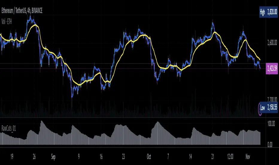
Trend Strength with Volatility and Volume [ST]Trend Strength with Volatility and Volume
Description in English:
This indicator combines market volatility and trading volume to measure the current trend strength. It helps identify when the trend is gaining or losing momentum.
Detailed Explanation:
Configuration:
Length: This input defines the period over which the moving average is calculated. The default value is 14.
MA Type: This input allows you to choose between a Simple Moving Average (SMA) and an Exponential Moving Average (EMA).
Volatility Length: This input defines the period over which the ATR (Average True Range) is calculated. The default value is 14.
Volume Length: This input defines the period over which the moving average of volume is calculated. The default value is 14.
Trend Strength Calculation:
Moving Average (MA): The script calculates the moving average of the closing price based on the selected type (SMA or EMA) and period.
Volatility (ATR): The ATR is used to measure market volatility over the specified period.
Volume MA: The script calculates the moving average of the trading volume based on the selected type (SMA or EMA) and period.
Trend Strength: The trend strength is calculated as the difference between the closing price and the moving average, divided by the volatility, and multiplied by the volume normalized by its moving average.
Plotting:
The trend strength is plotted as a line chart. Positive values indicate a strong upward trend, while negative values indicate a strong downward trend.
A horizontal line is added at the zero level to help identify the neutral point.
Indicator Benefits:
Trend Identification: Helps traders identify the strength of the current trend by combining price, volatility, and volume.
Visual Cues: Provides clear visual signals for trend strength, aiding in making informed trading decisions.
Customizable Parameters: Allows traders to adjust the length of the moving averages, ATR, and volume to suit different trading strategies and market conditions.
Justification of Component Combination:
Combining price, volatility, and volume provides a comprehensive measure of trend strength. This combination enhances the trader's ability to make informed decisions based on multiple market factors.
How Components Work Together:
The script calculates the moving average of the closing price and trading volume.
It measures market volatility using the ATR.
The trend strength is calculated by combining these components, providing a robust measure of the current trend's strength.
Título: Força da Tendência com Volatilidade e Volume
Descrição em Português:
Este indicador combina a volatilidade do mercado, medida pelo ATR (Average True Range), e o volume de negociações para medir a força da tendência atual. Ele ajuda a identificar quando a tendência está ganhando ou perdendo força.
Explicação Detalhada:
Configuração:
Comprimento: Este parâmetro define o período para o cálculo da média móvel. O valor padrão é 14.
Tipo de MA: Este parâmetro permite escolher entre uma Média Móvel Simples (SMA) e uma Média Móvel Exponencial (EMA).
Comprimento da Volatilidade: Este parâmetro define o período para o cálculo do ATR (Average True Range). O valor padrão é 14.
Comprimento do Volume: Este parâmetro define o período para o cálculo da média móvel do volume. O valor padrão é 14.
Cálculo da Força da Tendência:
Média Móvel (MA): O indicador calcula a média móvel do preço de fechamento com base no tipo selecionado (SMA ou EMA) e período.
Volatilidade (ATR): O ATR é usado para medir a volatilidade do mercado ao longo do período especificado.
Média Móvel do Volume: O indicador calcula a média móvel do volume de negociação com base no tipo selecionado (SMA ou EMA) e período.
Força da Tendência: A força da tendência é calculada como a diferença entre o preço de fechamento e a média móvel, dividida pela volatilidade e multiplicada pelo volume normalizado pela sua média móvel.
Plotagem:
A força da tendência é plotada como um gráfico de linhas. Valores positivos indicam uma forte tendência de alta, enquanto valores negativos indicam uma forte tendência de baixa.
Uma linha horizontal é adicionada no nível zero para ajudar a identificar o ponto neutro.
Benefícios do Indicador:
Identificação de Tendências: Este indicador ajuda os traders a identificar a força da tendência atual, combinando preço, volatilidade e volume.
Sinais Visuais Claros: Fornece sinais visuais claros para a força da tendência, facilitando a tomada de decisões informadas.
Parâmetros Personalizáveis: Os traders podem ajustar o comprimento das médias móveis, ATR e volume para se adequar a diferentes estratégias de negociação e condições de mercado.
Justificação da Combinação de Componentes:
A combinação de preço, volatilidade e volume fornece uma medida abrangente da força da tendência.
Isso melhora a capacidade dos traders de tomar decisões informadas com base em múltiplos fatores do mercado.
Como os Componentes Funcionam Juntos:
O indicador calcula a média móvel do preço de fechamento e do volume de negociação.
Mede a volatilidade do mercado usando o ATR.
A força da tendência é calculada combinando esses componentes, fornecendo uma medida robusta da força da tendência atual.
